Corfu Navision 2016, Data, Development Tips, Dimension, Excel, Functional Tips, How To, Information, Tip & Tricks

How to attach additional 6 Shortcut Dimensions to Dimension Set when copy data to Journal from Excel


In my previous post I explained how we can copy data to-and-fro between Excel and Navision. Also we saw the limitation of additional 6 Shortcut Dimensions neither can be exported nor imported back.

Today we will see solution to this limitation, as it is required from several customers and we keep getting request for same. The same reader for whom I have posted my previous post have requested similar need.

If you missed my previous post you can find here : Copying data to-and-fro between Excel & Navision

Let us see how we can get this part working, yes it will require a small customization to get this working. Below I explain the steps we require to achieve this.

My example refers to Table 81 & Page 39. You can do same with other Journals too.

We will Add Custom Fields for these additional 6 Shortcut Dimensions.


ExcelToNavJnl-8

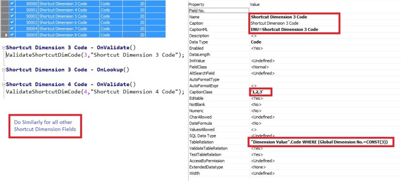
Add the Fields and write the above code to OnValidate trigger and set the Property accordingly for all of the 6 Shortcut Dimension Fields.

ExcelToNavJnl-9

Similarly add a piece of code to OnInsert trigger of the Table.

ExcelToNavJnl-10

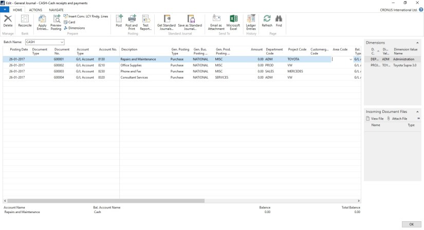
Add our newly created Fields to Page too.

Now Let us check if it works as expected.

ExcelToNavJnl-11


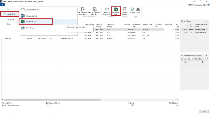
Perform the operation as in previous post, this time add the newly created fields for Dimensions as shown in above screen.

If you missed my previous post you can find here : Copying data to-and-fro between Excel & Navision

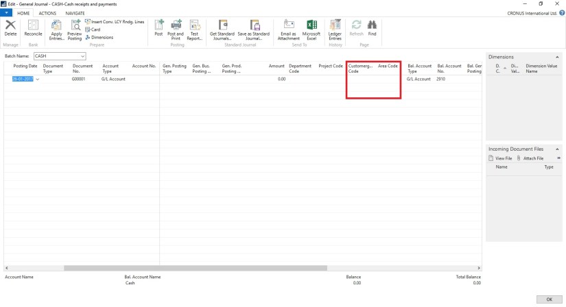
Export and Import back by adding value to these additional Dimensions 1 &2 is Global 3-6 is my additional Shortcut Dimensions, 7-8 I have not included as not setup in my database.

After importing back check the Dimensions and you will find due to above customization my all the Shortcut Dimensions are attached to Dimension Set Entry.
ExcelToNavJnl-12

Yes we are done.

I will come up with more information in my upcoming posts. Till then keep exploring and Learning.


Advertisement
Corfu Navision 2016, Data, Development Tips, Dimension, Excel, Functional Tips, How To, Information, Tip & Tricks

Copying data to-and-fro between Excel & Navision

ExcelToNavJnl

One of my reader has requested to show him how to export data from Nav Journal to Excel, perform correction and import back to Navision.

So let us see how can we perform this and what are the limitations.

Open the Journal in Navision.

Arrange and show all the Fields that you want to export to Excel on the page.

Fill some sample data. Say single line of Journal, way usually you do.

ExcelToNavJnl-2

Now Send to Excel using options shown in below screen.

ExcelToNavJnl-3

Data will get Exported to Excel.

Have you noticed something, with the data that got exported yo Excel?

Your 2 Additional Shortcut dimension was not Exported to Excel. Customer Group Code & Area Code, why?

Since these are not the actual fields in the table and it is calculated on Page level, so you will only be able to export Dim-1 & Dim-2 your Global Dimensions which is available as Field in the Table.

Make sure you enter Dimension Values in Capitals in Excel Columns.

ExcelToNavJnl-4

Now perform required changes to the Journal data.

Insert New Lines, Delete existing Lines or Edit existing Lines.

Make sure you don’t keep more than 30000 to 40000 lines, until this it works fine if more than this either performance is too slow or Navision gets hang while you copy back your data to Navision. Upto 40000 works fine have tested several time. Depending upon your system performance you can decide how much data will be ok for you.

ExcelToNavJnl-5

As we have seen above my 2 additional Dimensions is missing from the exported data. We need to match the columns what we have in our Excel and sequence. So we will hide/remove the additional columns from the Journal to match the sequence from Excel columns before we copy back our data from Excel to Navision.

ExcelToNavJnl-6

Select the Rows in excel containing you data excluding header columns and copy.

Return to your Journal and Paste as shown in above screen.

ExcelToNavJnl-7

Your modified data is imported back to the Journal in Navision.

Now perform the Journal action way you do normally.


Convert to PDF, Development Tips, Excel, How To, Information, Office Integration, Tip & Tricks, Word

Appending other information to Navision Reports

There is always requirement from many customers to Append information to the Navision Reports.

Recently one of my reader have requested me for any such functionality which can help him Append information from Word or Excel Files to Navision Reports.

While searching for solution for such requirement i came across this scope if we can do the same from outside Navision integrating the functionality with Navision.

Although i am not sure how much this post will answere to the requirement raised by my this reader but still this can be an work around to this requirement.

In my previous 2 posts i have answered this approach, Let us assemble all of them to provide solution to this requirement.

Please see my privious posts, i will not repeat already covered part in this post. Here is the link to those posts:

Converting Office Files into PDF from Navision

Merging PDF Files in Navision

In this post i will be using these functions discussed in above posts.

The Same Setup will be applicable to this post too.

PDFConvMerge-2-2

Since we are appending our other information to the Navision Report so we will be at First Step saving our Customer Sales Invoice to PDF.

Later some information which need to be appended to this report is in Word File the path of which is stored on Customer Card.

How to work with Converting Office file to PDF is already discussed in previous post Link shared above.

So Now we have Our Report in PDF and Additional information to be appended to Report is also in PDF. Now it will be easy for us to Merge both the File to have single PDF File.

How to Merge these files is also already discussed in my previous post. Link shared above.

Let us see how we can assemble above both functionality to get our required result.

Approach is very simple, i have created a button on Sales Invoice to Print the Report which performs above discussed process.

PDFConvMerge-5

On Sales Invoice Page I have added one Button which calls my Function to Print & Merge the document, it takes Invoice No & Sell-to Customer No. as a parameter.

PDFConvMerge-6

I have created a function to Save the output of Report to PDF, using standard functionality available in Navision.

PDFConvMerge-7

The PrintSalesInvoice function called from Sales Invoice Page with Invoice No & Sell-to Customer No.

This Function calls the SaveReportAsPDF explained above.

Converts the Office file that is attached on Custommer Card, discussed in previous post Link provided above.

Calls the MergePDFFiles, discussed in previous post Link provided above.

So Now at single click of Button entire task is done for us.

To keep it simple no additional checks and other routine tasks have been included like after task is completed clean up of all temporary files and moving the Result file to desired Location etc.

Now you know the logic so you can tweak the code accordingly to get the functionality working as per your requirement.

Thats all for this post. I will come up with more information in my up coming posts.

You keep you requirements posting to me, i will try my best to answer your queries in form of my future posts, at earliest possible from my end.

Till then kee exploring & Learning.

Development Tips, Email, Excel, How To, Information, Office Integration, Report, Server, Tip & Tricks

Export Data as CSV and send as Attachment to Mail

One of my Follower/Reader have requested for this post.

This post will explain the the below steps:

  • Export the data of table to csv file format. (I am using XMLPort you can use Excell Buffer or any other method to create the file)
  • Attach to Mail and Send.

Step 1.

Create a XMLPort as below.

CSVAttachment-1

Set the Property of XMLPort.

CSVAttachment-2

Set the Property of Integer Data Item.

CSVAttachment-3

Set the Property of Table DataItem for which data to be exported.

CSVAttachment-4

Set the Captions of the Columns in CSV file.

CSVAttachment-5

Write the code to transfer the value of Table columns.

You may find some extra code adjust accordingly as per your requirement.

CSVAttachment-6

Define a function to Setfilter for data to export.

Adjust the code as per your requirement.

CSVAttachment-7

CSVAttachment-8

Step 2.

Here is the function to Export the data to csv File using above created XMLPort.

This function Saves the file to Shared folder, if required you can use TEMPORARYPATH to save your File.

CSVAttachment-9

Step 3.

Send the File as Attachment to the Mail.

CSVAttachment-10

You make required adjustment as per your requirement.

Make sure in case you are using Shared Folder give necessary rights on folder to Service Account and operating User Accounts.

Please respond did you found useful this information.

Their are other ways to achive the same, this was readyly available with me as i have used in one of my project so shared the same.

Stay tuned for more details in my Up comming posts.

Data Model, Development Tips, Excel, How To, Information, Instalation & Configuration, Office Integration, PivotTable, Power View, PowerBI.com, PowerPivot

PowerPivot in Excel 2013

I started the series in End of September and Starting of October on PowerPivot, Power View, PivotTable & Reports but in-between the release of Navision 2016 all the topics got scattered between other posts and I didn’t ended the topic.

Here I present all the posts link at one place which you can use as table of content for easy access and to help if any one wish to start from beginning and learn all the features & Topic on same.

PowerPivot for Excel

Start the Power Pivot in Microsoft Excel add-in

Troubleshooting: Power Pivot Ribbon Disappears

PowerPivot Creating a Data Model in Excel 2013

Adding more tables to the Data Model using Existing Connection – In PowerPivot

Add relationships to Data Model in PowerPivot

How to add Filter for data retrieval in PowerPivot Data model.

Create a calculated column in PowerPivot

Creating My First Report using PowerPivot

Basics of Power Pivot for Excel – 2013

Add Slicers to PivotTables in PowerPivot

Power View in Excel 2013

Import data using copy and paste from Excel sheet or other source for PowerPivot Data Model.

Add Excel Sheet/Table to the PowerPivot Data Model

Add a relationship using Diagram View in Power Pivot

Extend the Data Model using calculated columns

Create a hierarchy in PowerPivot Data Model

Use hierarchies in PivotTables

Create a Power View report

Create a calculated field in PowerPivot

Set field defaults in PowerPivot

Set Table Behaviour in PowerPivot

Set Data Categories for fields in PowerPivot

I will come up with more details once I get some time to explore and find anything which I feel is good to share with the community.

Till then keep Learning, Exploring and Practicing.

Data Model, Development Tips, Excel, How To, PowerPivot

Set Data Categories for fields in PowerPivot

In order for Power View to dynamically create reports based on underlying data, such as location, fields that contain such data must be properly categorized.

Open the Excel Workbook we created in our earlier post. Create a Power View report

For the Olympics data, let’s specify the categories for a few fields.

  • In Power Pivot, select Hosts. Select the NOC_CountryRegion field. From Advanced -> Reporting Properties -> Data Category: click the arrow and select Country/Region from the list of available data categories, as shown in the following screen.

ExcelData-37

  • Return to Excel, and select the Power View sheet. Expand the Medals table in Power View Fields, and notice that the NOC_CountryRegion field now has a small globe icon beside it. The globe indicates that NOC_CountryRegion contains a geographic location, as shown in the following screen.

ExcelData-38

We’ll use that geographic location in an upcoming post. It’s time to save your work, review what you’ve learned, and then get ready to dive into the next post.

I will come up with more details in my next post. Till then Stay Tuned, Keep Learning & Practicing.

Data Model, Development Tips, Excel, How To, Power View, PowerPivot

Set Table Behaviour in PowerPivot

You can set the default table behaviour, which Power View uses to automatically create report labels for the table.

This becomes useful when you create visualizations from the same table, perhaps for many different reports.

Open the Excel Workbook we created in our earlier post. Create a Power View report

We use default table behaviour in the next few steps, so let’s set it now.

Open Medals Table in Data Model, select Advanced > Reporting Properties > Table Behaviour. A window appears where you can specify table behaviour.
ExcelData-33

  • In the Table Behavior window, the Row Identifier is the column that contains only unique keys and no blank values. This is often the table’s primary key, but not compulsory to be any other field which satisfy this property. You have to select a Row Identifier before making other selections in the window. Select MedalKey as the Row Identifier.
  • In the Keep Unique Rows section, select AthleteID.

Fields you select here have row values that should be unique, and should not be aggregated when creating Pivot Tables or Power View reports.
Note: If you have trouble with reports that don’t aggregate how you want them, make sure that the field you want to aggregate is not selected in the Keep Unique Rows fields.

  • For Default Label, select a key that should be used as a default report label. Select Sport.
  • For Default Image, leave the selection as [No Column Selected], since you haven’t added images yet. The Table Behavior window looks like the following screen.

ExcelData-34

  • On the Power View sheet in Excel, select the table you created in the previous post Set field defaults in PowerPivot
  • From the ribbon, select DESIGN -> Table -> Card.

ExcelData-35

  • The table you created changes into a collection of Cards; the data is the same, but the visualization of the data has changed. The table now looks like the following screen.

ExcelData-36

Notice that the Sport field is larger than the rest, and appears as a heading for each card. That’s because we set Sport as the Default Label in the Table Behavior window when we were in Power Pivot.

I will come up with more details in my upcoming posts. Till then Stay Tuned, Keep Learning & Practicing.

Data Model, Development Tips, Excel, How To, Power View, PowerPivot

Set field defaults in PowerPivot

When you set a default field set for a table, you can simply click that table in Power View, and the default set of fields is automatically added to a new report.

Open the Excel Workbook we created in our earlier post. Create a Power View report

In today’s post, we will learn how to set defaults for our workbook that will save our time when creating reports.

Steps to Create the Default Field Set for a table

  • Select the Medals table in Data View Mode from PowerPivot Manager.
  • From the Advanced tab, select Reporting Properties > Default Field Set. A window appears that lets you specify default fields for tables created using client tools such as Power View.
  • Select Sport, Event, EditionID, Athlete, and Medal in the left pane, and click Add -> to make them the default fields.

ExcelData-31

To see how this works, switch to the Power View sheet in Excel.

  • Click anywhere on the blank report canvas, to make sure you don’t have an existing visualization selected. Your Power View sheet currently only has one visualization, which is the map you created earlier in previous post. Create a Power View report
  • In the Power View Fields list, click the Medals table name. Power View creates a table and automatically adds the five default fields from the Medals table, in the order you specified, as shown in the following screen. Make sure you don’t click on the triangle beside Medals, if you do so the table simply expands, rather than adding a new table with default fields.

ExcelData-32

I will come up with more details on this topic in my upcoming posts. Till then Stay Tuned, Keep Learning and Practicing.

Data Model, Development Tips, Excel, How To, PowerPivot

Create a calculated field in PowerPivot

Open the Excel workbook which we used in our previous post on this topic. Olympics Excel Work book.

Select PowerPivot -> Manage

PowerPivot Window will open, If Calculation area not visible below table data as shown in below screen. Click Calculation Area button in Top Right Corner.

ExcelData-27

In the Calculation Area, select the cell directly below the Edition column. From the ribbon, select AutoSum > Distinct Count, as shown in the following screen.
ExcelData-28

Power Pivot automatically created the following DAX formula: Distinct Count of Edition:=DISTINCTCOUNT([Edition])

Additional calculations in AutoSum are just as easy, such as Sum, Average, Min, Max, and others.

Let’s calculate the percentage of all medals. In the formula bar, type the following DAX formula. IntelliSense provides available commands based on what you type, and you can press Tab to select the highlighted IntelliSense option. Percentage of All Medals:=[Count of Medal]/CALCULATE([Count of Medal],ALL(Medals))
ExcelData-29

When we return to Excel Sheet we can find these fields available in Medal Table. Shown in the right side of the screen above.

Let’s create a PivotTable from Medal Table. Our Pivot Table will be designed as below screen.
ExcelData-30

I will come up with more details inn my upcoming posts. Till then stay tuned, keep Learning and keep practicing.

Data Model, Excel, How To, PivotTable, Power View, PowerPivot

Create a Power View report

In the previous post, we created an Excel workbook with a PivotTable containing data about Olympic medals and events. If you didn’t saw the previous post you can access from here.

Use hierarchies in PivotTables

In this post, we will create a Power View report to visually represent the Olympics data.

In Excel, click INSERT > Reports > Power View Reports.
ExcelData-22

ExcelData-23

ExcelData-24
Select City from Host & Sport from Medal Table. Apply Count (Not Blank) to Sport Field using dropdown list next to Field Name.
ExcelData-25
From design switch the Visualization to Map.

On the map, blue circles of varying size indicate the number of different sport events held at each Olympic Host location.
ExcelData-26
Drag Season Field to Color area. This will add different colors for different Seasons. In our case summer/Winter Red/Blue colors.

Just in few clicks now we have a Power View report that visualizes the number of sporting events in various locations, using a map, color-coded based on season.

Will come with more details in my upcoming posts, till then stay tuned, keep learning and practicing.