Corfu Navision 2016, Functional Tips, How To, Information, Tip & Tricks

Create Production Orders for/from Sales Order

One of my reader have requested to demonstrate how he can create Sales Order which is directly associated with Sales Order.

Let us start with creating a Sales Order:

ProdOrder-1

Here you can see we don’t have Available Inventory to fulfil the demand of this Order.

ProdOrder-2

To fulfil the demand we will create Production Order for this Order.

Select Planning from Action TAB on Ribbon.

Sales Order Planning Window Opens, Select Create Production Order.

ProdOrder-3

Select the Status for Production Order as desired.

For Order Type you have 2 Options

  1. Item Order – Production Order is created for each Item on Lines
  2. Project Order – Single Production order for Entire Order

Select the desired option and respond to Yes.

ProdOrder-4

I have Selected Released & Project Order in my case.

ProdOrder-5

You can check that Quantity to be produced is reserved for this Order.

There could be the situation where you may have few Inventory available, in that case you need to reserve the quantity from Function before creating Production Order else all quantity will be created. In other case only short quantity will be a quantity of Production Order.

ProdOrder-6

Select the line from available lines in Item Ledger Entries (e.g. on hand inventory) and by using the ‘Reserve from Current Line’ function you can reserve those against the sales order line.  The ‘Reserved Quantity’ then gets updated and you can see the rest in the ‘Unreserved Quantity’ field.

ProdOrder-7

Although in this case entire line is already reserved from the Production Order.

But in case you want to reserve from any available Inventory in hand from Ledger entry.

This was one of the way how you can perform Creating Production Order and Reserving for Sales Order.

We can do the same by another way as below, directly creating Production Order for this Sales Order.

ProdOrder-8

Create a Production Order Select Source Type as Sales Header and Source No as Sales Order No.

Then Refresh the Production Order.

ProdOrder-9


ProdOrder-10


This way we can create and Reserve the Item for required demand.

I will come with more details in my upcoming posts.


Data Model, Development Tips, Excel, How To, PowerPivot

Create a calculated field in PowerPivot

Open the Excel workbook which we used in our previous post on this topic. Olympics Excel Work book.

Select PowerPivot -> Manage

PowerPivot Window will open, If Calculation area not visible below table data as shown in below screen. Click Calculation Area button in Top Right Corner.

ExcelData-27

In the Calculation Area, select the cell directly below the Edition column. From the ribbon, select AutoSum > Distinct Count, as shown in the following screen.
ExcelData-28

Power Pivot automatically created the following DAX formula: Distinct Count of Edition:=DISTINCTCOUNT([Edition])

Additional calculations in AutoSum are just as easy, such as Sum, Average, Min, Max, and others.

Let’s calculate the percentage of all medals. In the formula bar, type the following DAX formula. IntelliSense provides available commands based on what you type, and you can press Tab to select the highlighted IntelliSense option. Percentage of All Medals:=[Count of Medal]/CALCULATE([Count of Medal],ALL(Medals))
ExcelData-29

When we return to Excel Sheet we can find these fields available in Medal Table. Shown in the right side of the screen above.

Let’s create a PivotTable from Medal Table. Our Pivot Table will be designed as below screen.
ExcelData-30

I will come up with more details inn my upcoming posts. Till then stay tuned, keep Learning and keep practicing.

Data Model, Excel, How To, PivotTable, Power View, PowerPivot

Create a Power View report

In the previous post, we created an Excel workbook with a PivotTable containing data about Olympic medals and events. If you didn’t saw the previous post you can access from here.

Use hierarchies in PivotTables

In this post, we will create a Power View report to visually represent the Olympics data.

In Excel, click INSERT > Reports > Power View Reports.
ExcelData-22

ExcelData-23

ExcelData-24
Select City from Host & Sport from Medal Table. Apply Count (Not Blank) to Sport Field using dropdown list next to Field Name.
ExcelData-25
From design switch the Visualization to Map.

On the map, blue circles of varying size indicate the number of different sport events held at each Olympic Host location.
ExcelData-26
Drag Season Field to Color area. This will add different colors for different Seasons. In our case summer/Winter Red/Blue colors.

Just in few clicks now we have a Power View report that visualizes the number of sporting events in various locations, using a map, color-coded based on season.

Will come with more details in my upcoming posts, till then stay tuned, keep learning and practicing.

Data Model, Development Tips, Excel, How To, PowerPivot, Report

Create a hierarchy in PowerPivot Data Model

We will be using the Excel workbook we used in our earlier posts. Open the Excel file, you can find the link for download in my earlier posts or from blog Menu.

SharePath

Most Data Models include data that is inherently hierarchical. The Olympics data is also hierarchical. It’s helpful to understand the Olympics hierarchy, in terms of sports, disciplines, and events.

For each sport, there is one or more associated disciplines (sometimes there are many).

And for each discipline, there is one or more events (again, sometimes there are many events in each discipline).

The following Table illustrates the hierarchy.

ExcelData-13

In this post we will create two hierarchies within the Olympic data. Then use these hierarchies to see how hierarchies make organizing data easy in PivotTables and in Power View in upcoming posts.

Create a Sport hierarchy

In Power Pivot, switch to Diagram View. Expand the Events table so that you can more easily see all of its fields.

ExcelData-14

  • Press and hold Ctrl, and click the Sport, Discipline, and Event fields. With those three fields selected, right-click and select Create Hierarchy. A parent hierarchy node, Hierarchy 1, is created at the bottom of the table, and the selected columns are copied under the hierarchy as child nodes. Verify that Sport appears first in the hierarchy, then Discipline, then Event.

ExcelData-15

  • Double-click the title, Hierarchy1, and type SDE to rename your new hierarchy. You now have a hierarchy that includes Sport, Discipline and Event. Your Events table now looks like the above screen.
  • Still in Diagram View in Power Pivot, select the Hosts table and click the Create Hierarchy button in the table header, as shown in the following screen.

ExcelData-16

  • An empty hierarchy parent node appears at the bottom of the table.
  • Type Locations as the name for your new hierarchy.
  • There are many ways to add columns to a hierarchy. Drag the Season, City and NOC_CountryRegion fields onto the hierarchy name (in this case, Locations) until the hierarchy name is highlighted, then release to add them.
  • Right-click EditionID and select Add to Hierarchy. Choose Locations.
  • Ensure that your hierarchy child nodes are in order. From top to bottom, the order should be: Season, NOC, City, EditionID. If your child nodes are out of order, simply drag them into the appropriate ordering in the hierarchy. Your table should look like the above screen.

Your Data Model now has hierarchies that can be put to good use in reports. In the upcoming posts we will learn how these hierarchies can make our report creation faster, and more consistent.

Stay tuned for more details, will come up with usage of hierarchy in my upcoming post.

Till then keep learning & practicing.

Development Tips, Excel, How To, Office Integration, PowerPivot, Report

Create a calculated column in PowerPivot

If you have missed earlier post, please walkthrough them for better understanding from below links:

PowerPivot for Excel

PowerPivot Creating a Data Model in Excel 2013

Adding more tables to the Data Model using Existing Connection – In PowerPivot

Add relationships to Data Model in PowerPivot

How to add Filter for data retrieval in PowerPivot Data model.

In Power Pivot, you can use Data Analysis Expressions (DAX) to add calculations. In this task, I will add simple Excel Formula =ABS (Quantity) in Item Ledger Entry Sheet. You can add formulas either simple calculation from two fields or referencing from other tables and sheet. I will come with more details on this in separate post.

  • In the Power Pivot window, switch to Data View.
  • Select the Item Ledger Entry table/ sheet.
  • Click Design > Add.

PowerPivot-18

Alternatively you can Add by selecting Column, Right Click and choose Insert Column as you do in Excel.

New Column Will be Added.

  • In the formula bar above the table, type the following formula. AutoComplete helps you type the fully qualified names of columns and tables, and lists the functions that are available. You can also just click the column and Power Pivot adds the column name to the formula.

In my case it is =abs([Quantity])

  • When you have finished building the formula, press Enter to accept the formula.

Values are populated for all the rows in the calculated column. If you scroll down through the table, you will see that rows can have different values for this column, based on the data that is in each row.

Rename the column by right-clicking and selecting Rename Column.
PowerPivot-19

  • Type Sales Quantity, and then press Enter.

Below is the Screen after populating the value post formula application to Calculated Column.
PowerPivot-20

I will come up with more details in my upcoming post, Till then keep practicing and stay tuned for more details and updates on this topic.

Development Tips, Office Integration

Using Automation to Create a Graph in Microsoft Excel

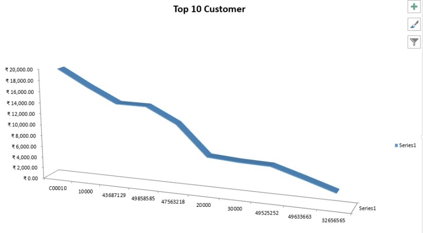
In this walkthrough, you will transfer data for top 10 Customers Sales Contribution to Microsoft Excel and create a graph.

This example shows how to handle enumerations by creating a graph in Excel that shows the distribution of Sales by Customer.

ExcelChart-1

You will run the codeunit directly from Object Designer. In a real application, you would call it from an appropriate place, such as from a menu or any other window.

About This Walkthrough

This walkthrough illustrates the following tasks:

  • Creating a codeunit that declares the Automation variables that are required for using Excel Automation.
  • Adding a function to calculate Top 10 Customers Sales Contribution.
  • Adding C/AL code to the codeunit to run the Automation object that opens Excel.
  • Adding C/AL code to the Automation codeunit to transfer data from a table record to Excel.
  • Adding C/AL code that creates a graph in Excel. 

Prerequisites 

To complete this walkthrough, you will need:

  • Microsoft Dynamics NAV 2015 with a developer license.
  • The CRONUS International Ltd. demo data company.
  • Microsoft Excel 2013 or Microsoft Excel 2010.

Creating the Codeunit and Declaring Variables

To create the codeunit and declare variables

  • To implement Automation in a codeunit, you define the Automation variables. To define an Automation variable, you specify an Automation server and the Automation object.
  • The language in the regional settings of your computer matches the language version of Microsoft Excel.
  • In Object Designer, choose Codeunit, and then choose the New button to create a new codeunit.
  • On the View menu, choose C/AL Globals.
  • On the Variables tab, add the following variables:

Note

For the Automation data type variables, the subtype Microsoft Excel 15.0/14.0 Object Library defines the Automation server, and the class specifies the Automation object of the Microsoft Excel 15.0/14.0 Object Library.

ExcelChart-2

Name DataType Subtype Length
xlApp Automation ‘Microsoft Excel 15.0 Object Library’.Application
xlBook Automation ‘Microsoft Excel 15.0 Object Library’.Workbook
xlSheet Automation ‘Microsoft Excel 15.0 Object Library’.Worksheet
xlChart Automation ‘Microsoft Excel 15.0 Object Library’.Chart
xlRange Automation ‘Microsoft Excel 15.0 Object Library’.Range
Cust Record Customer
Window Dialog
CustAmount Record Customer Amount
CustFilter Text
CustDateFilter Text 30
ShowType Option  [Sales (LCY),Balance (LCY)]
NoOfRecordsToPrint Integer
CustSalesLCY Decimal
CustBalanceLCY Decimal
MaxAmount Decimal
BarText Text 50
i Integer
TotalSales Decimal
TotalBalance Decimal
ChartType Option  [Bar chart,Pie chart]
ChartTypeNo Integer
ShowTypeNo Integer
ChartTypeVisible Boolean
Integer Record Integer
Customer Record Customer
CellNo1 Text 5
CellNo2 Text 5
  • Close the C/AL Globals window.

Adding the Code

Now you add the code for the codeunit.

To add the code

  • Add a Function to calculate Top 10 Customers Sales Contribution as:
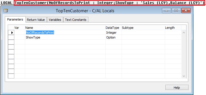
ExcelChart-3
Add code to it as:

I have not used all the values, just shown this way also you can think of while you design any such code & functions.

Window.OPEN(Text000);

i := 0;

Cust.RESET;

IF Cust.FINDSET THEN

REPEAT

Window.UPDATE(1,Cust.”No.”);

Cust.CALCFIELDS(“Sales (LCY)”,”Balance (LCY)”);

IF (Cust.”Sales (LCY)” <> 0) OR (Cust.”Balance (LCY)” <> 0) THEN

BEGIN

CustAmount.INIT;

CustAmount.”Customer No.” := Cust.”No.”;

IF ShowType = ShowType::”Sales (LCY)” THEN BEGIN

CustAmount.”Amount (LCY)” := -Cust.”Sales (LCY)”;

CustAmount.”Amount 2 (LCY)” := -Cust.”Balance (LCY)”;

END ELSE BEGIN

CustAmount.”Amount (LCY)” := -Cust.”Balance (LCY)”;

CustAmount.”Amount 2 (LCY)” := -Cust.”Sales (LCY)”;

END;

CustAmount.INSERT;

IF (NoOfRecordsToPrint = 0) OR (i < NoOfRecordsToPrint) THEN

i := i + 1

ELSE BEGIN

CustAmount.FIND(‘+’);

CustAmount.DELETE;

END;

TotalSales += Cust.”Sales (LCY)”;

TotalBalance += Cust.”Balance (LCY)”;

ChartTypeNo := ChartType;

ShowTypeNo := ShowType;

END;

UNTIL Cust.NEXT = 0;

CustSalesLCY := Cust.”Sales (LCY)”;

CustBalanceLCY := Cust.”Balance (LCY)”;

Window.CLOSE;

IF CustAmount.FIND(‘-‘) THEN

REPEAT

CustAmount.”Amount (LCY)” := -CustAmount.”Amount (LCY)”;

Customer.GET(CustAmount.”Customer No.”);

Customer.CALCFIELDS(“Sales (LCY)”,”Balance (LCY)”);

IF MaxAmount = 0 THEN

MaxAmount := CustAmount.”Amount (LCY)”;

CustAmount.”Amount (LCY)” := -CustAmount.”Amount (LCY)”;

UNTIL CustAmount.NEXT = 0;

  • In the C/AL Editor, make call to above function by adding the following code to the OnRun trigger.

CustAmount.DELETEALL;

TopTenCustomer(10,ShowType::”Sales (LCY)”,ChartType::”Bar chart”);

  • Create an instance of Excel by adding the following code.

CREATE(xlApp, FALSE, TRUE);

  • Add a new workbook to Excel.

xlBook := xlApp.Workbooks.Add(-4167);

xlSheet:= xlApp.ActiveSheet;

xlSheet.Name := ‘Top 10 Customer’;

The following describes the code:

    • In the first line, you use the Add method of the Workbooks collection to return a new workbook. The attribute -4167 is the enumerator value of worksheets as they apply to Workbook objects.
    • In the second line, you use the ActiveSheet property of the Application class to ensure that what is done next affects the active sheet of the new workbook.
    • In the third line, you use the Name property to name the sheet.

Transferring Data

To transfer the data, you must calculate the data and transfer the results of the calculation.

To transfer data

  • In the C/AL Editor, on the codeunit, use following code to transfer data of Top 10 Customers to Excel. To transfer the data to Microsoft Excel, add the following code.

CellNo1 := ‘A1’;

CellNo2 := ‘B1’;

IF CustAmount.FINDSET THEN

REPEAT

CellNo1 := INCSTR(CellNo1);

xlSheet.Range(CellNo1).Value := CustAmount.”Customer No.”;

CellNo2 := INCSTR(CellNo2);

xlSheet.Range(CellNo2).Value := ABS(CustAmount.”Amount (LCY)”);

UNTIL CustAmount.NEXT = 0;

  • The final step is to create the graph. You will use the ChartWizard method to create chart. This is a fast and simple way to do it. You can more tightly control the design of the graph by setting it up using the methods and properties of the various Chart objects, such as ChartArea and Legend.

Creating the Graph

The final step is to create the graph. You will use the ChartWizard method to create chart. This is a fast and simple way to do it. You can more tightly control the design of the graph by setting it up using the methods and properties of the various Chart objects, such as ChartArea and Legend.

To create the graph

  •   In the C/AL Editor, on the current codeunit, define a range for the data in the graph.

xlRange := xlSheet.Range(‘A2:’+FORMAT(CellNo2));

  • Add a new chart sheet and give it a name.xlChart.Name := ‘ Top 10 Customer – Graph’;

xlChart := xlBook.Charts.Add;

xlChart.Name := ‘ Top 10 Customer – Graph’;

  • Create the graph.

xlChart.ChartWizard(xlRange,-4101,7,2,1,0,1,’Top 10 Customer’);

The following table describes the optional arguments that are used in the ChartWizard method.

Argument Description Value in method call
Source The range that contains the source data for the new chart. xlRange – The object returned by xlSheet.Range(‘A2:C3’).
Gallery The chart type. -4101 – The enumerator for the Chart Shown above.
Format The option number for the built-in auto formats. 7
PlotBy An integer specifying whether the data for each series is in rows or columns. 2 – The enumerator for the xlRows XlRowCol enumerator.
CategoryLabels An integer specifying the number of rows or columns within the source range that contains category labels. 1 – There is one row with category labels (the department names).
SeriesLabels An integer specifying the number of rows or columns within the source range that contains series labels. 0 – There are no series labels in your data.
HasLegend TRUE to include a legend. 1
Title VARIANT with the title of the chart. You pass a string such as ‘Top 10 Customer’.
  • Make Excel visible by adding the following code.

xlApp.Visible := TRUE;

Excel produces a General Protection Fault error when you close a new Excel worksheet that is created when Excel is invisible. To resolve this, you can make Excel visible immediately after you create a new worksheet. You can also make Excel visible just before you create a new Excel worksheet and then make it invisible again immediately after creating the new Excel worksheet. In this case, you would add the following code.

xlApp.Visible := TRUE;

xlBook := xlApp.Workbooks.Open(FileName);

xlApp.Visible := FALSE;

  •  Clearing the Temp Table by adding the following code.

CustAmount.DELETEALL;

  • Complete code in OnRun trigger should look like below:

ExcelChart-4
Saving and Running the Codeunit

You can test the codeunit for creating the graph by running the codeunit from Object Designer.

To save and run a codeunit

  1. On the File menu, choose Save.
  2. In the Save As window, enter an ID and name, and then choose the OK
  3. In Object Designer, select the codeunit, and then choose the Run

The Microsoft Excel graph should appear. As show above in beginning of the post.

Note

If you get an error states Old format or invalid type library, then make sure that the language in the regional settings of your computer matches the language version of Microsoft Excel.

Below detailed reference to the values used in above code:


XlChartType

Name Value Description
xl3DArea -4098 3D Area.
xl3DAreaStacked 78 3D Stacked Area.
xl3DAreaStacked100 79 100% Stacked Area.
xl3DBarClustered 60 3D Clustered Bar.
xl3DBarStacked 61 3D Stacked Bar.
xl3DBarStacked100 62 3D 100% Stacked Bar.
xl3DColumn -4100 3D Column.
xl3DColumnClustered 54 3D Clustered Column.
xl3DColumnStacked 55 3D Stacked Column.
xl3DColumnStacked100 56 3D 100% Stacked Column.
xl3DLine -4101 3D Line.
xl3DPie -4102 3D Pie.
xl3DPieExploded 70 Exploded 3D Pie.
xlArea 1 Area
xlAreaStacked 76 Stacked Area.
xlAreaStacked100 77 100% Stacked Area.
xlBarClustered 57 Clustered Bar.
xlBarOfPie 71 Bar of Pie.
xlBarStacked 58 Stacked Bar.
xlBarStacked100 59 100% Stacked Bar.
xlBubble 15 Bubble.
xlBubble3DEffect 87 Bubble with 3D effects.
xlColumnClustered 51 Clustered Column.
xlColumnStacked 52 Stacked Column.
xlColumnStacked100 53 100% Stacked Column.
xlConeBarClustered 102 Clustered Cone Bar.
xlConeBarStacked 103 Stacked Cone Bar.
xlConeBarStacked100 104 100% Stacked Cone Bar.
xlConeCol 105 3D Cone Column.
xlConeColClustered 99 Clustered Cone Column.
xlConeColStacked 100 Stacked Cone Column.
xlConeColStacked100 101 100% Stacked Cone Column.
xlCylinderBarClustered 95 Clustered Cylinder Bar.
xlCylinderBarStacked 96 Stacked Cylinder Bar.
xlCylinderBarStacked100 97 100% Stacked Cylinder Bar.
xlCylinderCol 98 3D Cylinder Column.
xlCylinderColClustered 92 Clustered Cone Column.
xlCylinderColStacked 93 Stacked Cone Column.
xlCylinderColStacked100 94 100% Stacked Cylinder Column.
xlDoughnut -4120 Doughnut.
xlDoughnutExploded 80 Exploded Doughnut.
xlLine 4 Line.
xlLineMarkers 65 Line with Markers.
xlLineMarkersStacked 66 Stacked Line with Markers.
xlLineMarkersStacked100 67 100% Stacked Line with Markers.
xlLineStacked 63 Stacked Line.
xlLineStacked100 64 100% Stacked Line.
xlPie 5 Pie.
xlPieExploded 69 Exploded Pie.
xlPieOfPie 68 Pie of Pie.
xlPyramidBarClustered 109 Clustered Pyramid Bar.
xlPyramidBarStacked 110 Stacked Pyramid Bar.
xlPyramidBarStacked100 111 100% Stacked Pyramid Bar.
xlPyramidCol 112 3D Pyramid Column.
xlPyramidColClustered 106 Clustered Pyramid Column.
xlPyramidColStacked 107 Stacked Pyramid Column.
xlPyramidColStacked100 108 100% Stacked Pyramid Column.
xlRadar -4151 Radar.
xlRadarFilled 82 Filled Radar.
xlRadarMarkers 81 Radar with Data Markers.
xlStockHLC 88 High-Low-Close.
xlStockOHLC 89 Open-High-Low-Close.
xlStockVHLC 90 Volume-High-Low-Close.
xlStockVOHLC 91 Volume-Open-High-Low-Close.
xlSurface 83 3D Surface.
xlSurfaceTopView 85 Surface (Top View).
xlSurfaceTopViewWireframe 86 Surface (Top View wireframe).
xlSurfaceWireframe 84 3D Surface (wireframe).
xlXYScatter -4169 Scatter.
xlXYScatterLines 74 Scatter with Lines.
xlXYScatterLinesNoMarkers 75 Scatter with Lines and No Data Markers.
xlXYScatterSmooth 72 Scatter with Smoothed Lines.
xlXYScatterSmoothNoMarkers 73 Scatter with Smoothed Lines and No Data Markers.

expression .ChartWizard(Source, Gallery, Format, PlotBy, CategoryLabels, SeriesLabels, HasLegend, Title, CategoryTitle, ValueTitle, ExtraTitle)

expression A variable that represents a Chart object.

Parameters

Name Required/Optional Data Type Description
Source Optional Variant The range that contains the source data for the new chart. If this argument is omitted, Microsoft Excel edits the active chart sheet or the selected chart on the active worksheet.
Gallery Optional Variant One of the constants of XlChartType specifying the chart type.
Format Optional Variant The option number for the built-in autoformats. Can be a number from 1 through 10, depending on the gallery type. If this argument is omitted, Microsoft Excel chooses a default value based on the gallery type and data source.
PlotBy Optional Variant Specifies whether the data for each series is in rows or columns. Can be one of the following XlRowCol constants: xlRows or xlColumns. Values can be [1 or 2]
CategoryLabels Optional Variant An integer specifying the number of rows or columns within the source range that contain category labels. Legal values are from 0 (zero) through one less than the maximum number of the corresponding categories or series.
SeriesLabels Optional Variant An integer specifying the number of rows or columns within the source range that contain series labels. Legal values are from 0 (zero) through one less than the maximum number of the corresponding categories or series.
HasLegend Optional Variant True to include a legend.
Title Optional Variant The chart title text.
CategoryTitle Optional Variant The category axis title text.
ValueTitle Optional Variant The value axis title text.
ExtraTitle Optional Variant The series axis title for 3-D charts or the second value axis title for 2-D charts.

Remarks

If Source is omitted and either the selection isn’t an embedded chart on the active worksheet or the active sheet isn’t an existing chart, this method fails and an error occurs.

You can use other values from above table to create graph of your choice.

Development Tips

How to create and install a test certificate for the Microsoft Dynamics NAV Server computer

To start with this exercise you need to first create certificate and certificate revocation list, if not yet created refer to previous post.

Previous Step Link- How to create a root CA and a private key file by using the makecert.exe utility

Previous Step Link- How to create certificate revocation list for the root certification authority

Let’s start with this exercise:

  • At the command prompt, type the following command:

makecert -sk NavServiceCert -iv RootNavServiceCA.pvk -n “CN=NavServiceCert” -ic RootNavServiceCA.cer -sr localmachine -ss my -sky exchange -pe NavServiceCert.cer

Note

This command specifies the subject’s certificate name as NavServiceCert. You need this certificate name when you configure the Microsoft Dynamics NAV Windows client or Microsoft Dynamics NAV Web Server components.

Certificate-13

  • When you are prompted, enter the password that you used to create the root CA.
  • Select the Trusted Root Certificate Authorities node, and then refresh the snap-in.

You now have the NavServiceCert.cer certificate file in your temporary folder. The certificate is installed under the Personal node in the Certificates Snap-in.

Certificate-14
In next step we will now grant access to the certificate’s private key to the service account on computer running Microsoft Dynamics NAV Server.

Next Step Link- How to grant access to the certificate’s private key to the service account for the Microsoft Dynamics NAV Server computer

Development Tips

How to create a certificate revocation list for the root certification authority

To start with this exercise you need to first create certificate, if not yet created refer to previous post.

Previous Step Link- How to create a root CA and a private key file by using the makecert.exe utility

Let’s start with this exercise:

  • On the computer running Microsoft Dynamics NAV Server, create a temporary folder to use when you work with certificates.
  • Open the command prompt as follows:
    • If you have Visual Studio installed on your computer, choose Start, choose All Programs, choose Microsoft Visual Studio 2012, choose Visual Studio Tools, and then right-click Visual Studio Command Prompt and choose Run as Administrator.
    • If you have the Windows SDK installed on your computer, choose Start, choose All Programs, choose Microsoft Windows SDK, and then right-click Windows SDK Command Prompt (2010) (or CMD Shell) and choose Run as Administrator.
  • At the command prompt, locate the temporary directory.
  • At the command prompt, type the following command:

makecert -crl -n “CN=RootNavServiceCA” -r -sv RootNavServiceCA.pvk RootNavServiceCA.crl

  • When you are prompted, enter the password that you used to create the root CA.

Certificate-9
The RootNavServiceCA.crl certificate revocation file is saved in your temporary folder.
Certificate-10
Now we will install the certificate revocation list on the computer running Microsoft Dynamics NAV Server

  • In the Certificates snap-in, in the left pane of MMC, expand the Certificates (Local Computer) node.
  • Expand the Trusted Root Certification Authorities node, right-click the Certificates subfolder, select All Tasks, and then choose Import.
  • In the Certificate Import Wizard, on the Welcome page, choose Next.
  • On the File to Import page, choose Browse.
  • In the File Type field, select Certificate Revocation List (*.crl).
  • Browse to the location of the RootNavServiceCA.crl file, select the file, and then choose Open.
  • On the File to Import page, choose Next.
  • On the Certificate Store page, accept the default selection, and then choose Next.
  • On the Completing the Certificate Import Wizard page, choose Finish.

Certificate-11

  • Select the Trusted Root Certificate Authorities node, and then refresh the snap-in.

A Certificate Revocation List folder that contains the RootNavServiceCA.crl file has been created.
Certificate-12
In next step we will now create and install a test certificate on computer running Microsoft Dynamics NAV Server.

Next Step Link- How to create and install a test certificate for the Microsoft Dynamics NAV Server computer

Development Tips

How to create a root CA and a private key file by using the makecert.exe utility

We will follow below step to create a certificate for Microsoft Dynamics Server. Then we will implement the same for login from WAN to access Navision using Windows and Web Clients.

  • On the computer running Microsoft Dynamics NAV Server, create a temporary folder to use when you work with certificates.
  • Open the command prompt as follows:
    • If you have Visual Studio installed on your computer, choose Start, choose All Programs, choose Microsoft Visual Studio 2012, choose Visual Studio Tools, and then right-click Visual Studio Command Prompt and choose Run as Administrator.
    • If you have the Windows SDK installed on your computer, choose Start, choose All Programs, choose Microsoft Windows SDK, and then right-click Windows SDK Command Prompt (2010) (or CMD Shell) and choose Run as Administrator.
  • At the command prompt, locate the temporary directory.
  • Type the following command.

makecert -n “CN=RootNavServiceCA” -r -sv RootNavServiceCA.pvk RootNavServiceCA.cer

Certificate-4

  • When you are prompted, enter a password.
    • You need this password to create the service certificate.
  • The RootNavServiceCA.cer certificate file and the RootNavServiceCA.pvk private key are saved in your temporary folder.

Certificate-5

Now we will use the Certificates snap-in to install the root CA on the computer running Microsoft Dynamics NAV Server

  • Start the Certificates snap-in for MMC on the computer running Microsoft Dynamics NAV Server, and then add the Certificates snap-in.
  • In the Certificates snap-in dialog box, choose Computer account, and then choose Next.
  • In the Select Computer pane, choose Local computer: (the computer this console is running on), and then choose Finish.
  • Choose OK to close the Add or Remove Snap-ins dialog box.
  • In the left pane of MMC, expand the Certificates (Local Computer) node.

Certificate-2

Certificate-3

  • Expand the Trusted Root Certification Authorities node, right-click the Certificates subfolder, select All Tasks, and then choose Import.

Certificate-6

  • In the Certificate Import Wizard, on the Welcome page, choose Next.
  • On the File to Import page, choose Browse.
  • Browse to the location of the RootNavServiceCA.cer certificate file, select the file, and then choose Open.
  • On the File to Import page, choose Next.
  • On the Certificate Store page, accept the default selection, and then choose Next.
  • On the Completing the Certificate Import Wizard page, choose Finish.

Certificate-7

The RootNavServiceCA certificate is now visible in the list of trusted root CAs.

Certificate-8

In next step we will now create a certificate revocation list for the root certification authority and then install the certificate revocation list on the computer running Microsoft Dynamics NAV Server.

A certificate revocation list is required because WCF applications check the revocation list when validating certificates.

Next Step Link- How to create a certificate revocation list for the root certification authority

Functional Tips

Create a Sales Invoice for a new Customer

In this session we will create a sales invoice for a new customer (Customer we don’t have in our Master).

To follow Step by Step you need to do a small setup:

Open the User Personalization and Set your Profile ID as below:

SINewCustomer-1

Select your Profile as “SMALL BUSINESS

Your Role Center will look like below:

SINewCustomer-2

  • On the Role Center, choose Ongoing Sales Invoices to open the list of ongoing sales Invoices.
  • On the Home tab, in the New group, choose New to create a new sales invoice.
  • In the Customer Name field, type the name of the new customer, and then press Enter or Tab to leave the field

Create the sales invoice for the new customer.

Notice that some fields are marked with red asterisks to tell which fields must be filled.

SINewCustomer-3

  • In the pop-up dialog, choose Yes to create the new customer
  • In the Templates window, select Customer DOMESTIC (or as desired), and then choose the OK button.

SINewCustomer-4

  • The Customer Card window opens in edit mode. Choose the OK button to close it.

SINewCustomer-5

  • The page closes and focus is back on the sales invoice that is now updated with the customer data.
  • In the Sales Invoice window, on the Lines FastTab, create a new line:

         Enter some line data for example : Item No.: 1001, Quantity: 10

  • On the Home tab, in the Posting group, choose Post.
  • Choose Yes.

SINewCustomer-6

  • Choose No to review the posted sales invoice, as of now we don’t require.

Helpful where we require instant Customer registration for recording the Orders. Later we will fill out rest of the details regarding Customer.