Data Model, Development Tips, Excel, How To, PowerPivot, Report

Create a hierarchy in PowerPivot Data Model

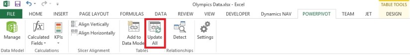
We will be using the Excel workbook we used in our earlier posts. Open the Excel file, you can find the link for download in my earlier posts or from blog Menu.

SharePath

Most Data Models include data that is inherently hierarchical. The Olympics data is also hierarchical. It’s helpful to understand the Olympics hierarchy, in terms of sports, disciplines, and events.

For each sport, there is one or more associated disciplines (sometimes there are many).

And for each discipline, there is one or more events (again, sometimes there are many events in each discipline).

The following Table illustrates the hierarchy.

ExcelData-13

In this post we will create two hierarchies within the Olympic data. Then use these hierarchies to see how hierarchies make organizing data easy in PivotTables and in Power View in upcoming posts.

Create a Sport hierarchy

In Power Pivot, switch to Diagram View. Expand the Events table so that you can more easily see all of its fields.

ExcelData-14

  • Press and hold Ctrl, and click the Sport, Discipline, and Event fields. With those three fields selected, right-click and select Create Hierarchy. A parent hierarchy node, Hierarchy 1, is created at the bottom of the table, and the selected columns are copied under the hierarchy as child nodes. Verify that Sport appears first in the hierarchy, then Discipline, then Event.

ExcelData-15

  • Double-click the title, Hierarchy1, and type SDE to rename your new hierarchy. You now have a hierarchy that includes Sport, Discipline and Event. Your Events table now looks like the above screen.
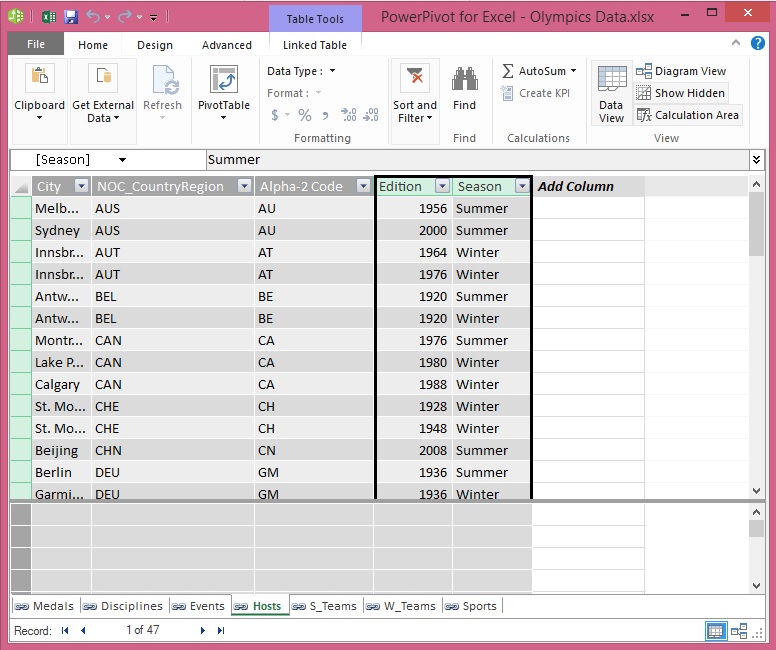
  • Still in Diagram View in Power Pivot, select the Hosts table and click the Create Hierarchy button in the table header, as shown in the following screen.

ExcelData-16

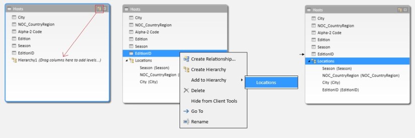
  • An empty hierarchy parent node appears at the bottom of the table.
  • Type Locations as the name for your new hierarchy.
  • There are many ways to add columns to a hierarchy. Drag the Season, City and NOC_CountryRegion fields onto the hierarchy name (in this case, Locations) until the hierarchy name is highlighted, then release to add them.
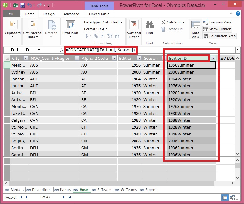
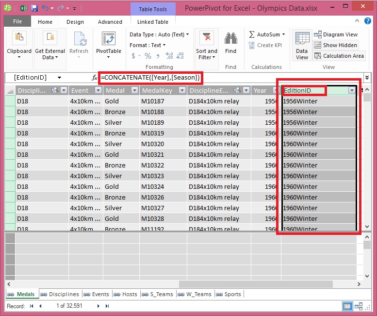
  • Right-click EditionID and select Add to Hierarchy. Choose Locations.
  • Ensure that your hierarchy child nodes are in order. From top to bottom, the order should be: Season, NOC, City, EditionID. If your child nodes are out of order, simply drag them into the appropriate ordering in the hierarchy. Your table should look like the above screen.

Your Data Model now has hierarchies that can be put to good use in reports. In the upcoming posts we will learn how these hierarchies can make our report creation faster, and more consistent.

Stay tuned for more details, will come up with usage of hierarchy in my upcoming post.

Till then keep learning & practicing.

Advertisement
Data Model, Development Tips, Excel, How To, PowerPivot, Report

Extend the Data Model using calculated columns

Recall from my previous post Add a relationship using Diagram View in Power Pivot

Which I have left with below note. I will be continuing from where I left my previous post.

It’s nice when the data in your Data Model has all the fields necessary to create relationships, and mash up data to visualize in Power View or PivotTables. But tables aren’t always so cooperative, so in today’s post will describe how to create a new column, using DAX that can be used to create a relationship between tables.

Open the Olympics Excel sheet which we used in our previous post.

ExcelData-7
Delete the column EditionID from sheet Medals & Hosts Table/Sheet.
ExcelData-8

After deleting the Column EditionID from Table/Sheet Select Update All in Ribbon from PowerPivot Tab. This will update the column in Data Model.

Since we are going to learn creating relationship on calculated fields.

In Hosts, we can create a unique calculated column by combining the Edition field (the year of the Olympics event) and the Season field (Summer or Winter). In the Medals table there is also an Edition field and a Season field, so if we create a calculated column in each of those tables that combines the Edition and Season fields, we can establish a relationship between Hosts and Medals. The following screen shows the Hosts table, with its Edition and Season fields selected
ExcelData-9

Select the Hosts table in Power Pivot. Adjacent to the existing columns is an empty column titled Add Column. Power Pivot provides that column as a placeholder. There are many ways to add a new column to a table in Power Pivot, one of which is to simply select the empty column that has the title Add Column.

In the formula bar, type the following DAX formula. The CONCATENATE function combines two or more fields into one. As you type, AutoComplete helps you type the fully qualified names of columns and tables, and lists the functions that are available. Use tab to select AutoComplete suggestions. You can also just click the column while typing your formula, and Power Pivot inserts the column name into your formula.

=CONCATENATE([Edition],[Season])

When you finish building the formula, press Enter to accept it.

Values are populated for all the rows in the calculated column. If you scroll down through the table, you see that each row is unique – so we’ve successfully created a field that uniquely identifies each row in the Hosts table. Such fields are called a primary key.

Let’s rename the calculated column to EditionID. You can rename any column by double-clicking it, or by right-clicking the column and choosing Rename Column. When completed, the Hosts table in Power Pivot looks like the following screen.
ExcelData-10

Next let’s create a calculated column in Medals that matches the format of the EditionID column we created in Hosts, so we can create a relationship between them.

When you created a new column, Power Pivot added another placeholder column called Add Column. Next we want to create the EditionID calculated column, so select Add Column. In the formula bar, type the following DAX formula and press Enter.

=CONCATENATE([Year],[Season])

Rename the column by double-clicking CalculatedColumn1 and typing EditionID.
ExcelData-11

Next let’s use the calculated columns we created to establish a relationship between Hosts and Medals.

In the Power Pivot window, select Home > View > Diagram View from the ribbon.

Drag the EditionID column in Medals to the EditionID column in Hosts. Power Pivot creates a relationship between the tables based on the EditionID column, and draws a line between the two columns, indicating the relationship.
ExcelData-12

Now you can see the relationship between Host & Medal table is established on calculated field EditionID in both the tables.

Stay tuned for more details on this topic. I will come up with next step in this series in my upcoming post.

Till then keep learning & practicing.

Data Model, Development Tips, Excel, How To, PowerPivot, Report

Add Excel Sheet/Table to the PowerPivot Data Model

Download the Excel file from the link provided in previous post.

Import data using copy and paste from Excel sheet or other source for PowerPivot Data Model.

Open the Workbook:

ExcelData-3

Select sheet one by one and Add to Data model of PowerPivot.

ExcelData-4

Make sure all Table/Sheet is added to Data Model of PowerPivot.

I have create a sample Excel File for you which you can down load from the Shared Path using link: http://1drv.ms/1GpZFd4

This file have couple of sheets having data related to Olympics which I have compiled from MS Office support site.

You can find the link on the Menu of my blogsite too to access the shared files.

I will be using this file for couple of walkthrough in my upcoming posts.

Data Model, Development Tips, Excel, PowerPivot

Import data using copy and paste from Excel sheet or other source for PowerPivot Data Model.

You can copy & Paste data from an Excel workbook, or import data from a table on a web page, or any other source from which we can copy and paste into Excel. In the following steps, you add the data from a table.

  • Insert a new Excel worksheet, and give it the name desired any meaningful name that describes the data.
  • Select and copy the data, including the table headers.
  • In Excel, place your cursor in cell A1 of the above created worksheet and paste the data.
  • Format the data as a table. You press Ctrl + T to format the data as a table, or from HOME > Format as Table. Since the data has headers, select My table has headers in the Create Table window that appears.

ExcelData-1

  • Name the table. In TABLE TOOLS > DESIGN > Properties locate the Table Name field, and type desired name.

ExcelData-2

  • Format your data using Excel std. formatting tool.
  • Save the workbook.This file have couple of sheets having data related to Olympics which I have compiled from MS Office support site.
  • You can find the link on the Menu of my blogsite too to access the shared files.
  • I have create a sample Excel File for you which you can down load from the Shared Path using link: http://1drv.ms/1GpZFd4

I will be using this file for couple of walkthrough in my upcoming posts.

Development Tips, Excel, How To, Office Integration, PowerPivot, Report

How to add Filter for data retrieval in PowerPivot Data model.

Recall from previous posts we have added Item Ledger Entry Table to our Data Model of PowerPivot.

Adding more tables to the Data Model using Existing Connection – In PowerPivot

Add relationships to Data Model in PowerPivot

My requirement is to retrieve only records related to Sales.

We will apply filter on Entry Type field to value [1]-[Sales] this way Item Leger Entry Sheet will have only Sales Data.

To do this we will add this filter to the query used for data retrieval.
PowerPivot-15

Select the Sheet for table – Item Ledger Entry from bottom.

Click on Design Tab on Top.

Now From Ribbon choose Table Properties.

PowerPivot-16

Select Query Editor from Switch to.

Add the Filter to your query.

Save your Query.

PowerPivot-17

From Home Tab, Select Refresh from Ribbon.

On Success completion Close the window.

Now your Item Ledger Entry is populated with Fresh data as per the modified Query.

I.e: All Entries which have Entry Type = 1 [Sales].

I will come up with more details in my upcoming post, till then keep practicing and stay tuned for future updates & posts on this topic.

Development Tips, Excel, How To, Office Integration, Report

Add relationships to Data Model in PowerPivot

You can systematically create table relationships for all new tables that you import. If you’re sharing the workbook with colleagues, having predefined relationships will be appreciated if they don’t know the data as well as you do.

When creating relationships manually, you will work with two tables at a time.

For each table, you’ll choose columns that tell Excel how to look up/ join related rows in another table.

Recall from my previous posts I will be continuing the example from using same Data Model

PowerPivot Creating a Data Model in Excel 2013

Adding more tables to the Data Model using Existing Connection – In PowerPivot

With your Data model sheet opened
PowerPivot-14
Click on Diagram View in Upper Right Side as highlighted in above screenshot.

Window will switch to Diagram View as shown in above screenshot, showing all the tables available in the Data model.

Click No_ in Customer Table and Drag to Item Ledger Entry Table and release the mouse button pointing to Source No_ field, you will see the Link is Established between these two tables showing the Link via Arrow line.

Repeat above step again between Item->No_ and Item Ledger Entry -> Item No_ fields.

Now we have Established connection between these three tables Customer, Item & Item Ledger Entry.

I will come up with more option on this topic in my next post, till then start practicing and stay tuned.

Development Tips, Excel, How To, Office Integration, PowerPivot, Report

Adding more tables to the Data Model using Existing Connection – In PowerPivot

For Introduction please see PowerPivot for Excel

Recall from my earlier post we have created a connection to SQL Navision Database in my previous post.

PowerPivot Creating a Data Model in Excel 2013

I will be modifying same connection to include more tables to the Data model.
PowerPivot-10

Click on PowerPivot-> Manage.

From the PowerPivot Sheet click on Existing Connections.

This will open Connection Window Listing all available connection to PowerPivot for this Sheet.

Double Click the Connection in my case Nav2015DB_SQL_Connection.
PowerPivot-6

Select first option as we used in previous post and then Next for next Step.
PowerPivot-11
Select Item & Item Ledger Entry Tables and then Finish to import Data to the Sheet.
PowerPivot-12
On Success Click Close to return to Data Model Sheets.
PowerPivot-13

You will find two new sheets have been added to PowerPivot Sheet.

I will come up with more option on this topic in my next post, till then start practicing and stay tuned for more details & Updates on this topic.

Development Tips, Excel, How To, Office Integration, PowerPivot, Report

PowerPivot Creating a Data Model in Excel 2013

Before you can create a PivotTable, you’ll need some data. Let’s get some data from the Navision database.

In Excel, open a blank workbook.

PowerPivot-1

PowerPivot-2

You have several options for getting data from no of sources.

Recall from my earlier post where we accessed data using web service in Excel.

Viewing Page Data in Excel Using PowerPivot (OData)

Let us see what other options are available to us.
PowerPivot-3

In today’s Example I will be connecting with SQL but will access Navision 2015 Database.

Follow the Steps below:
PowerPivot-4

Give meaningful name to your connection in my case I have used Nav2015DB_SQL_Connection.

Select the SQL Server to which you wish to connect in my case I have used INDEL-AXT5283N1, basically this is the SQL Server installed on my Laptop.
PowerPivot-5

Specify the Login method, I am using Windows Authentication, if required you can use SQL Server Authentication. In later case you will have to specify your User Name & Password.

Select the Database to Connect, I have selected Demo Database NAV (8-0) Std. Database for Navision 2015.

Click the Test Connection button, If everything is ok you will get Connection Succeed Message, as shown in above screen shot.

Press Next for next step.
PowerPivot-6

In this screen you have option to either import data from Tables and Views or you can Write Query to fetch data for import.

In my case for this example I am importing data from tables.

Select option – Select from a list of tables and views to choose the data to import and Press Next for next step.
PowerPivot-7

I have Selected two Tables Cust. Ledger Entry & Customer.

Select Related Tables button ensure to select if any other tables related to this Table.

In my case not applicable. Click Finish to add data to the Data Model/ Import the data of these two tables.
PowerPivot-8
Select Close to return to Data Sheet imported after this operation.
PowerPivot-9
Here you see your Data for these two tables have been imported in two sheets.

What happened?

You might not have realized it yet, but you’ve just created a data model. It’s created automatically when you import or work with multiple tables simultaneously in the same PivotTable report. The model is mostly transparent in Excel, but you can view and modify it directly using the Power Pivot add-in. In Excel, the presence of a data model is evident when you see a collection of tables in the PivotTable Fields list. There are several ways to create a model.

I will come up with more details in my next post.