Development Tips, Excel, How To, PowerPivot, Report

Add Slicers to PivotTables in PowerPivot

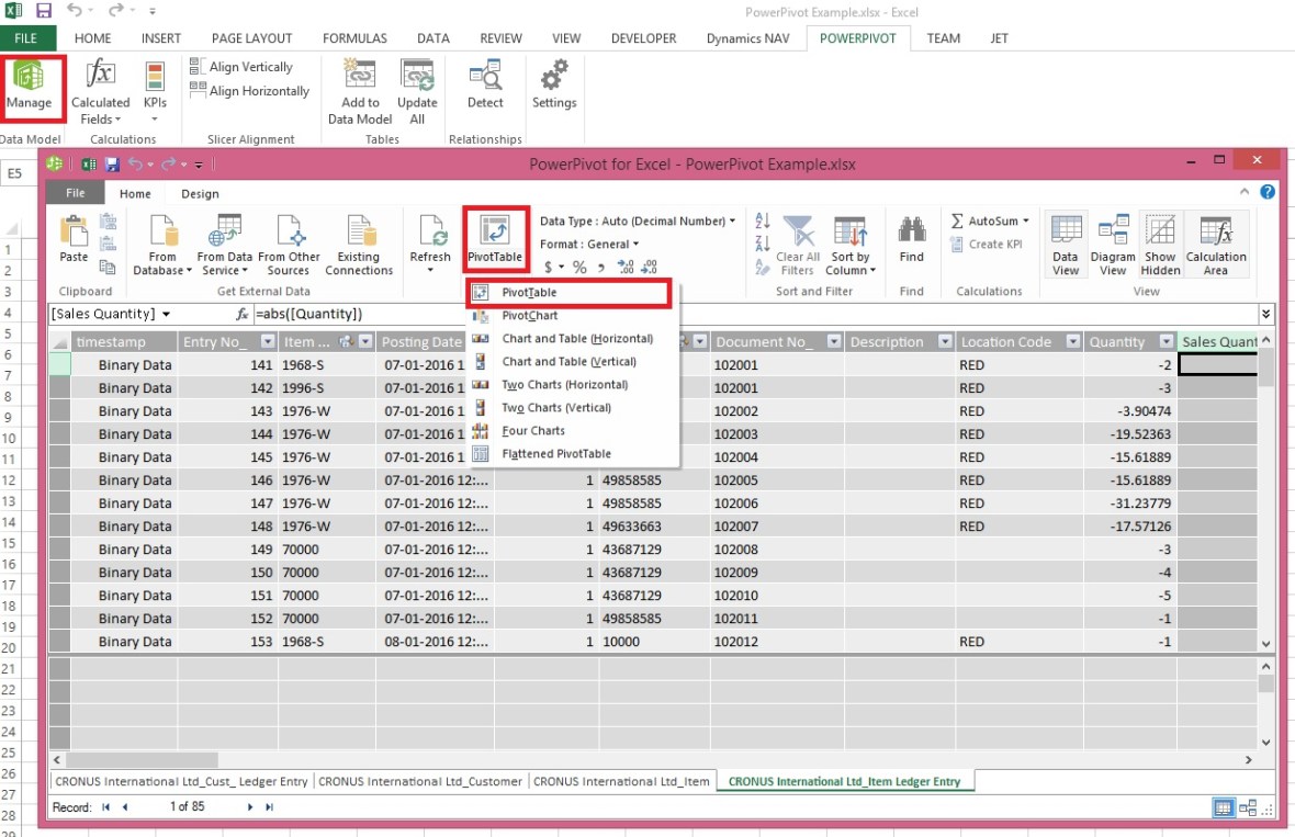
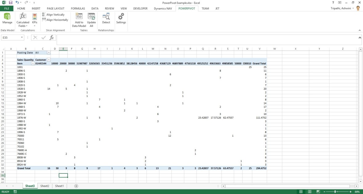
Recall from my earlier post Creating My First Report using PowerPivot in which we created a Items Vs Customer Sales matrix report.

I am going to use same report to demonstrate how we can add slicer to this report.

Slicers are one-click filtering controls that narrow the portion of a data set shown in PivotTables and PivotCharts. Slicers can be used in both Microsoft Excel workbooks and PowerPivot workbooks, to interactively filter and analyze data.
PowerPivot-30

Open the report we created in our previous post.

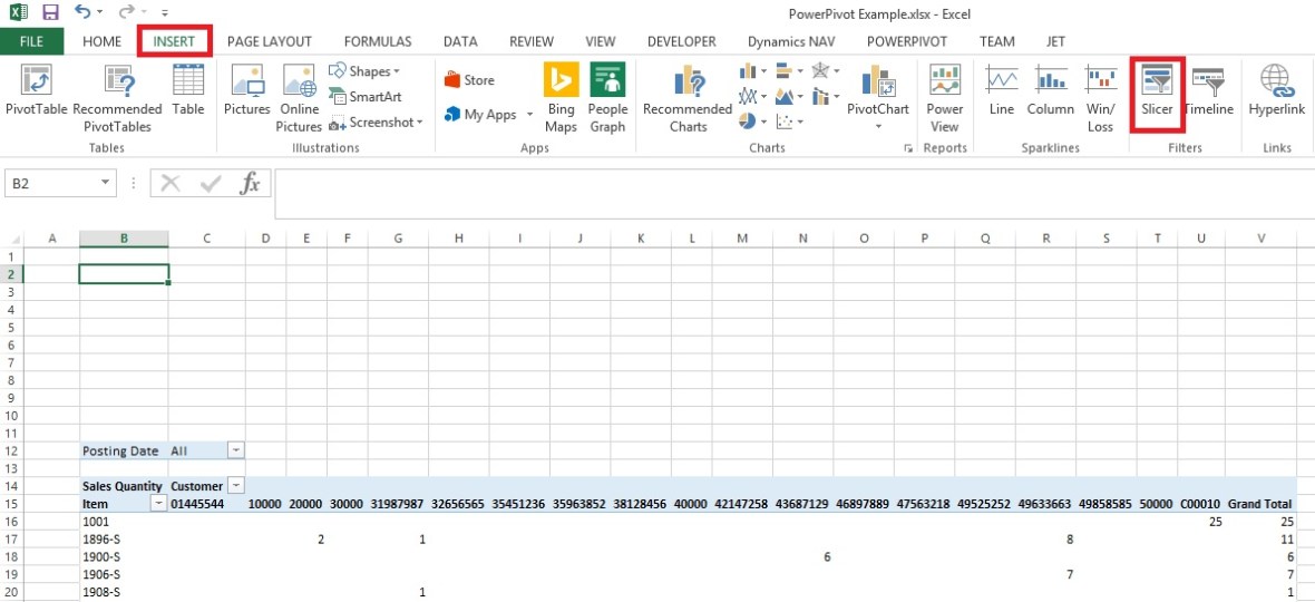
From Insert Tab select Slicer in the ribbon.
PowerPivot-31

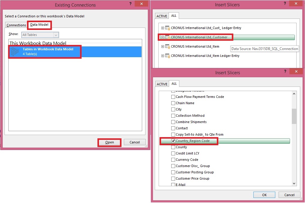
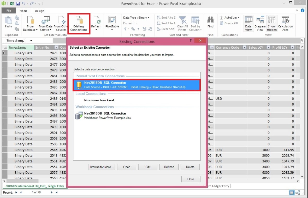
Choose the source Connection/Data model and respond Open.

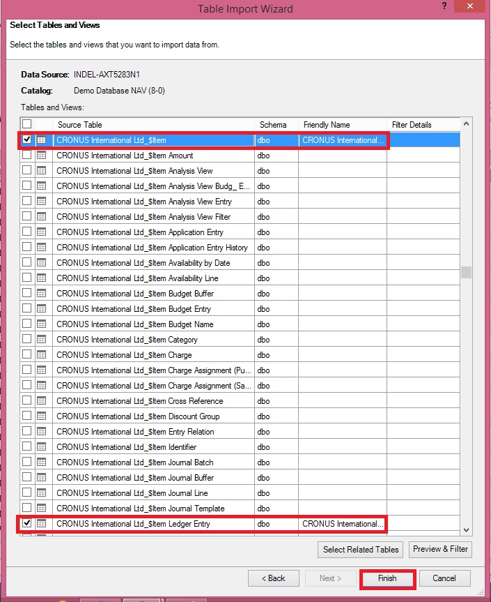
Select the Customer Table.

Select the Country/Region Code field and OK.
PowerPivot-32

A Slicer will be added to the sheet.

Re-size to fit and drag the Slicer to position at desired location on sheet.

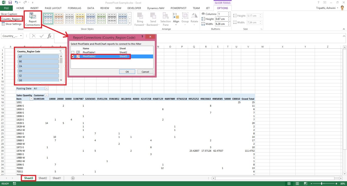
You can give desired Caption to your Slicer by editing the Slicer Caption.

Most important is to select the pivot table on which this Slicer will operate.

Select Report Connection, and from preceding window select the PivotTable.
PowerPivot-33
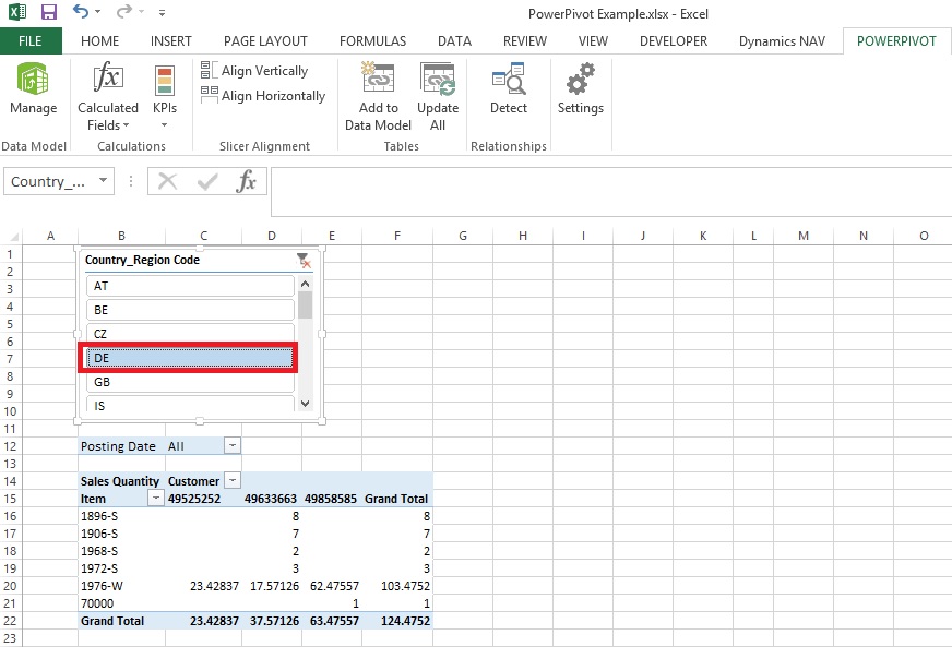
Above is the screenshot with applied filter on Country/Region Code = DE.

Stay tuned to know more options, I will come up with more details in my upcoming posts.

Till then keep practicing.

Awards

Achievments in Sep 2015

Dear Friends,

Today I am not writing any blog, wanted to share status as usually I do in every month as my first post.

I was awarded with Top 10 Blogger  in July month and my Rank was 6, in Aug moved to Rank 3.

This month in September I was busy with my some projects and travelling where I got less chance to write more posts. However managed to remain at Rank 4.

September was dedicated to Reporting tools mostly my posts were on Jet Reports and Power Pivot.

I stepped in blogging world 3 months ago, on 27 June 2015 I published my first post.

During this period I published almost 144 posts, most of them were more on technical side, Development Tips & Tricks.

Being a technical what I learned in past 10 years want to share with you all.

Achievment1
Achievment2
Achievment3
Achievment4
Achievment5

Stay tuned Follow the blog, Register to Feeds, Like the Facebook Page, Connect with Google + Page, Connect with Dynamics NAV Community, Connect with Twitter and Join on LinkedIn to remain updated about new posts. If you are technical don’t miss to get connected by any medium. I will make sure you keep getting good and useful stuffs.

I have created one Group on LinkedIn  also this month started Hike Group , join them so that we can discuss on some good topics where you can participate & are free to express your views and review others view.

Together we can learn from each other, no one is perfect in this world, its never late for learning.

Please participate and suggest topics, which you wish to see  on this blog. During this period I received request from many of you and tried to fulfil few requests. Request which yet I have not responded doesn’t mean I am not considering, I will make sure those too get posted at earliest.

After full day hectic schedule hardly I am able to takeout 2 hrs. for this task.

I will keep serving the community on my full strength.

See you all via my next post soon.

Excel, PowerPivot

Basics of Power Pivot for Excel – 2013

Dear friends, I have published couple of posts on this topic. I will be adding more advanced features and details related to this in my upcoming posts.

For your ready reference below I present Links to those posts.

PowerPivot for Excel

Start the Power Pivot in Microsoft Excel add-in

Troubleshooting: Power Pivot Ribbon Disappears

PowerPivot Creating a Data Model in Excel 2013

Adding more tables to the Data Model using Existing Connection – In PowerPivot

Add relationships to Data Model in PowerPivot

How to add Filter for data retrieval in PowerPivot Data model.

Create a calculated column in PowerPivot

Creating My First Report using PowerPivot

In Excel 2013, PowerPivot and Power View are no longer separate add-ins that need to be downloaded and installed. These add-ins are natively included.

PowerPivot in Excel 2013 is functionally very similar to the PowerPivot add-in for Excel 2010.

PowerPivot is an add-in that lets end users gather, store, model, and analyze large amounts of data in Excel. Power View provides intuitive data visualization of PowerPivot models and SQL Server Analysis Services (SSAS) tabular mode databases.

If you’re unfamiliar with either PowerPivot or Power View, I encourage you to first review my previous post links provided above to understand the basics.

Some parts of the PowerPivot architecture is embedded inside of Excel 2013.

  • The PowerPivot version in Excel 2013 no longer uses a separate PowerPivot Fields list. Instead, the built-in PivotTable Fields list is used. This means that some capabilities from the Excel 2010 add-in (e.g., searching for fields by name, creation of slicers from the field list, surfacing of column descriptions when hovering over a field) are no longer available.
  • Workbooks with PowerPivot models are no longer limited to 2GB in size in Excel 2013. However, the 2GB limit still applies to workbooks that will be published to SharePoint.
  • In Excel 2013, a refresh of a PivotTable or PivotChart will, by default, initiate a refresh of the underlying data connections in the Data Model. This is very different from Excel 2010, where a PivotTable refresh only re-queries the model. The new refresh behaviour can be changed by clicking Connections on the Data tab, selecting Properties, and clearing the Refresh this connection on Refresh All check box.
  • Stay tuned for more information on this topic. Till then keep practicing & exploring.
  • In Excel 2013, a Power View “report” is a worksheet rather than an .rdlx file. There’s no concept of multiple report views. Instead, multiple Power View worksheets can be created within a single Excel workbook.

Stay tuned for more information on this topic. Till then keep practicing & exploring.

Development Tips, Excel, How To, PowerPivot

Troubleshooting: Power Pivot Ribbon Disappears

In rare cases, the Power Pivot ribbon will disappear from the menu if Excel determines that the add-in is destabilizing to Excel. This might occur if Excel closes unexpectedly while the Power Pivot window is open. To restore the Power Pivot menu, do the following:

  • Go to File > Options > Add-Ins.

In the Manage box, click Disabled Items > Go
PowerPivot-29

  • Select Microsoft Office Power Pivot in Microsoft Excel 2013 and then click Enable.

If the previous steps do not restore the Power Pivot ribbon, or if the ribbon disappears when you close and reopen Excel, try the following:

  • Close Excel.
  • Point to Start > Run and then type regedit.
  • In Registry Editor, expand HKEY_CURRENT_USER > Software > Microsoft > Office > 15.0 > User Settings.
  • Right-click PowerPivotExcelAddin and then click Delete.
  • Scroll back up to the top of Registry Editor.
  • Expand HKEY_CURRENT_USER > Software > Microsoft > Office > Excel > Addins.
  • Right-click PowerPivotExcelClientAddIn.NativeEntry.1 and then click Delete.
  • Close Registry Editor.
  • Open Excel.
  • Enable the add-in using the steps at the top of this article.
Development Tips, Excel, How To, PowerPivot

Start the Power Pivot in Microsoft Excel add-in

Power Pivot in Microsoft Excel 2013 is an add-in you can use to perform powerful data analysis in Excel. The add-in is built into Excel, but by default, it’s not enabled. Here’s how you enable Power Pivot before using it for the first time.

  • Go to File > Options > Add-Ins.

In the Manage box, click COM Add-ins> Go
PowerPivot-26

  • Check the Microsoft Office Power Pivot in Microsoft Excel 2013 box, and then click OK. If you have other versions of the Power Pivot add-in installed, those versions are also listed in the COM Add-ins list. Be sure to select the Power Pivot add-in for Excel.

PowerPivot-27
The ribbon now has a Power Pivot tab
PowerPivot-28

Development Tips, Excel, How To, Office Integration, PowerPivot, Report

Creating My First Report using PowerPivot

In my earlier posts we have created the Data model for Analysis.

If you missed them you can follow below links to refresh all information.

PowerPivot for Excel

PowerPivot Creating a Data Model in Excel 2013

Adding more tables to the Data Model using Existing Connection – In PowerPivot

Add relationships to Data Model in PowerPivot

How to add Filter for data retrieval in PowerPivot Data model.

Create a calculated column in PowerPivot

We have learned basic actions, let’s create our first Report.

I will be creating Pivot Matrix Customer Vs Item Sales.

Open the Excel in which we created our Data model and imported our table data.
PowerPivot-21
Select PivotTable From Ribbon under Home Tab.
PowerPivot-22

Select New Worksheet or Existing Worksheet as per the case.
PowerPivot-23
You will see a Pivot is inserted, in right side you will find all the tables available in the Data model of this Worksheet.
PowerPivot-24

Design the Pivot as above screenshot.
The output of this report will be as below if executed without Date Filter.
PowerPivot-25
I will come up with more details and features of PowerPivot in my upcoming posts. Till then keep practicing and stay tuned for more details on this topic.

Development Tips, Excel, How To, Office Integration, PowerPivot, Report

Create a calculated column in PowerPivot

If you have missed earlier post, please walkthrough them for better understanding from below links:

PowerPivot for Excel

PowerPivot Creating a Data Model in Excel 2013

Adding more tables to the Data Model using Existing Connection – In PowerPivot

Add relationships to Data Model in PowerPivot

How to add Filter for data retrieval in PowerPivot Data model.

In Power Pivot, you can use Data Analysis Expressions (DAX) to add calculations. In this task, I will add simple Excel Formula =ABS (Quantity) in Item Ledger Entry Sheet. You can add formulas either simple calculation from two fields or referencing from other tables and sheet. I will come with more details on this in separate post.

  • In the Power Pivot window, switch to Data View.
  • Select the Item Ledger Entry table/ sheet.
  • Click Design > Add.

PowerPivot-18

Alternatively you can Add by selecting Column, Right Click and choose Insert Column as you do in Excel.

New Column Will be Added.

  • In the formula bar above the table, type the following formula. AutoComplete helps you type the fully qualified names of columns and tables, and lists the functions that are available. You can also just click the column and Power Pivot adds the column name to the formula.

In my case it is =abs([Quantity])

  • When you have finished building the formula, press Enter to accept the formula.

Values are populated for all the rows in the calculated column. If you scroll down through the table, you will see that rows can have different values for this column, based on the data that is in each row.

Rename the column by right-clicking and selecting Rename Column.
PowerPivot-19

  • Type Sales Quantity, and then press Enter.

Below is the Screen after populating the value post formula application to Calculated Column.
PowerPivot-20

I will come up with more details in my upcoming post, Till then keep practicing and stay tuned for more details and updates on this topic.

Development Tips, Excel, How To, Office Integration, PowerPivot, Report

How to add Filter for data retrieval in PowerPivot Data model.

Recall from previous posts we have added Item Ledger Entry Table to our Data Model of PowerPivot.

Adding more tables to the Data Model using Existing Connection – In PowerPivot

Add relationships to Data Model in PowerPivot

My requirement is to retrieve only records related to Sales.

We will apply filter on Entry Type field to value [1]-[Sales] this way Item Leger Entry Sheet will have only Sales Data.

To do this we will add this filter to the query used for data retrieval.
PowerPivot-15

Select the Sheet for table – Item Ledger Entry from bottom.

Click on Design Tab on Top.

Now From Ribbon choose Table Properties.

PowerPivot-16

Select Query Editor from Switch to.

Add the Filter to your query.

Save your Query.

PowerPivot-17

From Home Tab, Select Refresh from Ribbon.

On Success completion Close the window.

Now your Item Ledger Entry is populated with Fresh data as per the modified Query.

I.e: All Entries which have Entry Type = 1 [Sales].

I will come up with more details in my upcoming post, till then keep practicing and stay tuned for future updates & posts on this topic.

Development Tips, Excel, How To, Office Integration, Report

Add relationships to Data Model in PowerPivot

You can systematically create table relationships for all new tables that you import. If you’re sharing the workbook with colleagues, having predefined relationships will be appreciated if they don’t know the data as well as you do.

When creating relationships manually, you will work with two tables at a time.

For each table, you’ll choose columns that tell Excel how to look up/ join related rows in another table.

Recall from my previous posts I will be continuing the example from using same Data Model

PowerPivot Creating a Data Model in Excel 2013

Adding more tables to the Data Model using Existing Connection – In PowerPivot

With your Data model sheet opened
PowerPivot-14
Click on Diagram View in Upper Right Side as highlighted in above screenshot.

Window will switch to Diagram View as shown in above screenshot, showing all the tables available in the Data model.

Click No_ in Customer Table and Drag to Item Ledger Entry Table and release the mouse button pointing to Source No_ field, you will see the Link is Established between these two tables showing the Link via Arrow line.

Repeat above step again between Item->No_ and Item Ledger Entry -> Item No_ fields.

Now we have Established connection between these three tables Customer, Item & Item Ledger Entry.

I will come up with more option on this topic in my next post, till then start practicing and stay tuned.

Development Tips, Excel, How To, Office Integration, PowerPivot, Report

Adding more tables to the Data Model using Existing Connection – In PowerPivot

For Introduction please see PowerPivot for Excel

Recall from my earlier post we have created a connection to SQL Navision Database in my previous post.

PowerPivot Creating a Data Model in Excel 2013

I will be modifying same connection to include more tables to the Data model.
PowerPivot-10

Click on PowerPivot-> Manage.

From the PowerPivot Sheet click on Existing Connections.

This will open Connection Window Listing all available connection to PowerPivot for this Sheet.

Double Click the Connection in my case Nav2015DB_SQL_Connection.
PowerPivot-6

Select first option as we used in previous post and then Next for next Step.
PowerPivot-11
Select Item & Item Ledger Entry Tables and then Finish to import Data to the Sheet.
PowerPivot-12
On Success Click Close to return to Data Model Sheets.
PowerPivot-13

You will find two new sheets have been added to PowerPivot Sheet.

I will come up with more option on this topic in my next post, till then start practicing and stay tuned for more details & Updates on this topic.