Development Tips, Excel, How To, Office Integration, PowerPivot, Report

Create a calculated column in PowerPivot

If you have missed earlier post, please walkthrough them for better understanding from below links:

PowerPivot for Excel

PowerPivot Creating a Data Model in Excel 2013

Adding more tables to the Data Model using Existing Connection – In PowerPivot

Add relationships to Data Model in PowerPivot

How to add Filter for data retrieval in PowerPivot Data model.

In Power Pivot, you can use Data Analysis Expressions (DAX) to add calculations. In this task, I will add simple Excel Formula =ABS (Quantity) in Item Ledger Entry Sheet. You can add formulas either simple calculation from two fields or referencing from other tables and sheet. I will come with more details on this in separate post.

  • In the Power Pivot window, switch to Data View.
  • Select the Item Ledger Entry table/ sheet.
  • Click Design > Add.

PowerPivot-18

Alternatively you can Add by selecting Column, Right Click and choose Insert Column as you do in Excel.

New Column Will be Added.

  • In the formula bar above the table, type the following formula. AutoComplete helps you type the fully qualified names of columns and tables, and lists the functions that are available. You can also just click the column and Power Pivot adds the column name to the formula.

In my case it is =abs([Quantity])

  • When you have finished building the formula, press Enter to accept the formula.

Values are populated for all the rows in the calculated column. If you scroll down through the table, you will see that rows can have different values for this column, based on the data that is in each row.

Rename the column by right-clicking and selecting Rename Column.
PowerPivot-19

  • Type Sales Quantity, and then press Enter.

Below is the Screen after populating the value post formula application to Calculated Column.
PowerPivot-20

I will come up with more details in my upcoming post, Till then keep practicing and stay tuned for more details and updates on this topic.

Development Tips, Excel, How To, Office Integration, PowerPivot, Report

How to add Filter for data retrieval in PowerPivot Data model.

Recall from previous posts we have added Item Ledger Entry Table to our Data Model of PowerPivot.

Adding more tables to the Data Model using Existing Connection – In PowerPivot

Add relationships to Data Model in PowerPivot

My requirement is to retrieve only records related to Sales.

We will apply filter on Entry Type field to value [1]-[Sales] this way Item Leger Entry Sheet will have only Sales Data.

To do this we will add this filter to the query used for data retrieval.
PowerPivot-15

Select the Sheet for table – Item Ledger Entry from bottom.

Click on Design Tab on Top.

Now From Ribbon choose Table Properties.

PowerPivot-16

Select Query Editor from Switch to.

Add the Filter to your query.

Save your Query.

PowerPivot-17

From Home Tab, Select Refresh from Ribbon.

On Success completion Close the window.

Now your Item Ledger Entry is populated with Fresh data as per the modified Query.

I.e: All Entries which have Entry Type = 1 [Sales].

I will come up with more details in my upcoming post, till then keep practicing and stay tuned for future updates & posts on this topic.

Development Tips, Excel, How To, Office Integration, Report

Add relationships to Data Model in PowerPivot

You can systematically create table relationships for all new tables that you import. If you’re sharing the workbook with colleagues, having predefined relationships will be appreciated if they don’t know the data as well as you do.

When creating relationships manually, you will work with two tables at a time.

For each table, you’ll choose columns that tell Excel how to look up/ join related rows in another table.

Recall from my previous posts I will be continuing the example from using same Data Model

PowerPivot Creating a Data Model in Excel 2013

Adding more tables to the Data Model using Existing Connection – In PowerPivot

With your Data model sheet opened
PowerPivot-14
Click on Diagram View in Upper Right Side as highlighted in above screenshot.

Window will switch to Diagram View as shown in above screenshot, showing all the tables available in the Data model.

Click No_ in Customer Table and Drag to Item Ledger Entry Table and release the mouse button pointing to Source No_ field, you will see the Link is Established between these two tables showing the Link via Arrow line.

Repeat above step again between Item->No_ and Item Ledger Entry -> Item No_ fields.

Now we have Established connection between these three tables Customer, Item & Item Ledger Entry.

I will come up with more option on this topic in my next post, till then start practicing and stay tuned.

Development Tips, Excel, How To, Office Integration, PowerPivot, Report

Adding more tables to the Data Model using Existing Connection – In PowerPivot

For Introduction please see PowerPivot for Excel

Recall from my earlier post we have created a connection to SQL Navision Database in my previous post.

PowerPivot Creating a Data Model in Excel 2013

I will be modifying same connection to include more tables to the Data model.
PowerPivot-10

Click on PowerPivot-> Manage.

From the PowerPivot Sheet click on Existing Connections.

This will open Connection Window Listing all available connection to PowerPivot for this Sheet.

Double Click the Connection in my case Nav2015DB_SQL_Connection.
PowerPivot-6

Select first option as we used in previous post and then Next for next Step.
PowerPivot-11
Select Item & Item Ledger Entry Tables and then Finish to import Data to the Sheet.
PowerPivot-12
On Success Click Close to return to Data Model Sheets.
PowerPivot-13

You will find two new sheets have been added to PowerPivot Sheet.

I will come up with more option on this topic in my next post, till then start practicing and stay tuned for more details & Updates on this topic.

Development Tips, Excel, How To, Office Integration, PowerPivot, Report

PowerPivot Creating a Data Model in Excel 2013

Before you can create a PivotTable, you’ll need some data. Let’s get some data from the Navision database.

In Excel, open a blank workbook.

PowerPivot-1

PowerPivot-2

You have several options for getting data from no of sources.

Recall from my earlier post where we accessed data using web service in Excel.

Viewing Page Data in Excel Using PowerPivot (OData)

Let us see what other options are available to us.
PowerPivot-3

In today’s Example I will be connecting with SQL but will access Navision 2015 Database.

Follow the Steps below:
PowerPivot-4

Give meaningful name to your connection in my case I have used Nav2015DB_SQL_Connection.

Select the SQL Server to which you wish to connect in my case I have used INDEL-AXT5283N1, basically this is the SQL Server installed on my Laptop.
PowerPivot-5

Specify the Login method, I am using Windows Authentication, if required you can use SQL Server Authentication. In later case you will have to specify your User Name & Password.

Select the Database to Connect, I have selected Demo Database NAV (8-0) Std. Database for Navision 2015.

Click the Test Connection button, If everything is ok you will get Connection Succeed Message, as shown in above screen shot.

Press Next for next step.
PowerPivot-6

In this screen you have option to either import data from Tables and Views or you can Write Query to fetch data for import.

In my case for this example I am importing data from tables.

Select option – Select from a list of tables and views to choose the data to import and Press Next for next step.
PowerPivot-7

I have Selected two Tables Cust. Ledger Entry & Customer.

Select Related Tables button ensure to select if any other tables related to this Table.

In my case not applicable. Click Finish to add data to the Data Model/ Import the data of these two tables.
PowerPivot-8
Select Close to return to Data Sheet imported after this operation.
PowerPivot-9
Here you see your Data for these two tables have been imported in two sheets.

What happened?

You might not have realized it yet, but you’ve just created a data model. It’s created automatically when you import or work with multiple tables simultaneously in the same PivotTable report. The model is mostly transparent in Excel, but you can view and modify it directly using the Power Pivot add-in. In Excel, the presence of a data model is evident when you see a collection of tables in the PivotTable Fields list. There are several ways to create a model.

I will come up with more details in my next post.

Development Tips, Excel, How To, Jet Reports, Office Integration, Report

Other options for creating Report in Jet

Jet Report

Report Wizard

An entire report can be created from a single table using the Report Wizard. The Report Wizard allows data to be grouped, filtered, sorted, subtotaled, and formated.


Report Builder

The Report Builder creates reports based on Jet Data Views.  Jet Data Views define table relationships, available fields, field captions, and table captions for a particular reporting area, such as sales, inventory, payroll, etc.  Jet Data Views can be created using the Data View Creator.

Before Using the Report Builder

Before you use the Report Builder you will need to import or create data views and categories.

A set of data views for Dynamics NAV can be found on Jet Web Site you can access the same from here. You can also click on the Download Data Views link within the Report Builder.

After downloading the file, you should open the .zip folder and extract the data view category (.jdc) file.

Importing Data Views and Categories

To import data views and categories, go to the Data Source Settings and select File -> Import -> Data View Categories.


Table Builder

An entire report can be created from a single or more table using the Report Wizard. The Table Wizard allows data to be grouped, filtered, sorted, subtotaled, and formated.


Browser

Provides browsing window to Select Tables and Fields, using which you can directly create an NL/ NF Function with their parameters and arguments.


This way I reach to end of my Jet Report Introduction Series. In future I will keep adding more details.


Development Tips, Excel, How To, Jet Reports, Office Integration, Report

How to Use the Jet Report Scheduler

Overview

The Jet Scheduler is a powerful tool that allows users to schedule reports to be automatically run by the Windows Task Scheduler. The user can also control where the output file is saved to, if the report should be emailed once it has been generated, and the output format of the report.

Creating a New Scheduled Task

To set up a scheduled report, open the report in Excel, click the Jet ribbon, and click the Schedule button.

JetSchedule-1

Click the New Task… button to schedule a new task.

JetSchedule-2

The Scheduled Task window will now appear.

Reports Tab

JetSchedule-3

The Reports tab contains general information about the scheduled task.

  • Task Name: This represents the name of the task as it will appear in the Scheduled Task window to the user.
  • Run All Reports in a Folder: This button will enable the user to schedule all Jet Reports in a full to be run
  • Run a Single Report: This button will enable the user to schedule a single Jet Report to be run
  • Input: This represents the folder and file name of the report that will be run
  • Output: This represents the folder and file name of where the finished report will be saved

Schedule Tab

JetSchedule-4

This tab will define the frequency of how often the report will be run as well as if the task is currently disabled and if the report should be run when the user is logged off.

The available options for the frequency are:

  • Once: The report will only be run one time
  • Daily: The report will be run every day (it is possible to set on the next tab the number of days to wait between runs)
  • Weekly: The report will be run every week (it is possible to set on the next tab the days of the week for the report to be run on)
  • Monthly: The report will be run every month (it is possible to set on the next tab the months for the report to run on and the days of the month for the report to be run on)
  • When Idle: The report will run every time that the computer goes into idle mode
  • At Startup: The report will be run each time that the computer is turned on
  • At Logon: The report will be run each time that the user logs on to the computer

Frequency Tab

JetSchedule-5

The name of this tab will change depending on the frequency specified on the Schedule tab.

In the screenshot above a Weekly frequency has been specified.

  • Start Date and Time: This represents the first date that the report will run and the time that it will run for this and subsequent schedules
  • Weeks between report runs: This specifies how many weeks the Scheduler will wait between report runs before running the report again
  • Days to run report: This represents the days of the week that the report is scheduled to run on

Email Tab
JetSchedule-6
The Email tab allows the user to define who the report will be sent to if emailing is desired.

  • Send email: If this box is checked it will enable the report to be emailed to recipients
  • Mail properties: This dropdown will allow the user to specify whether the report will be emailed using Outlook or a generic SMTP protocol. SMTP must be configured in the Jet Essentials Application Settings in order for it to be used.
  • Message: This allows the user to specify a custom subject or body to be sent as part of the email
  • Attach report to email: If this box is checked the report will be attached to the email. If the box is unchecked the report will not be attached. This can be used as a type of notification when used in conjunction with the subject and body of the email to allow a user to know that the report has been run
  • Recipients: Email addresses will be specified here for all recipients of the report. Email addresses should be separated by a semi-colon.
  • Get recipients from Excel Named Range: It is possible to also define the email addresses in the report itself and then assign an Excel named range to the cell(s). If there are named ranges in the report then they will appear in the dropdown below the checkbox. The Output tab allows the user to define how the file should be saved once it is finished running. This tab also enabled the user to turn on logging to troubleshoot errors with the Scheduler process as well as use Batch File Generation for the reports.

Output Tab
The Output tab allows the user to define how the file should be saved once it is finished running. This tab also enabled the user to turn on logging to troubleshoot errors with the Scheduler process as well as use Batch File Generation for the reports.

JetSchedule-7

  • Output Format: This dropdown list will allow the user to define the format of the finished report. The available options are:
    • Jet Workbook: This will save the report as a normal Excel file with all Jet Reports functions still in the report
    • Values Only Workbook: This will save the report as an Excel file with all Jet Reports functions removed. The recipient would not be able to refresh the report as it will be a static Excel file
    • Web Page: This will save the report as a HTML file with a single sheet. This should be used when there is a single sheet in the report
    • Web Page by Sheet: This will save the report as a HTML file with multiple sheets embedded in it. This should be used when there are multiple sheets in a report
    • PDF: This will save the report as a PDF file (if your version of Excel supports that ability – Excel 2007 and higher)

Remain tuned for more details, I will come up with more details and features in my upcoming posts.

Development Tips, Excel, How To, Jet Reports, Office Integration, Report

Snippets in Jet Report

Snippets are small, reusable report parts that can be shared between Jet users.

Configuring the Snippet Folder and Sharing Snippets

Snippets are stored in the “Jet Reports Snippets” folder located in your My Documents directory.

This location can be changed in the Application Settings.  Each snippet is stored in a *.snippet file.  To share snippets, copy the snippet files from one user’s snippet directory to another’s.  Close and open the Snippets window and the newly added snippets will become available.

Snippet-1

Creating and Using a Snippet

Creating a Snippet

To create a snippet, open the Snippet tool.  Highlight the range of cells containing the piece of functionality for which to make a snippet.  Then, click the New Snippet button in the Snippet tool.

I have created a simple Report for Active Customers, which Lists all the customers where Blocked = ‘’

Snippet-2

We want to save this as a snipped so that any user can reuse it if required.

Snippet-3

  • Click the Snippet Button
  • Select the range of cells you want to save as snippet.
  • In Snippet Window click the New Snippet
  • Give the meaningful name to your Snippet.

Using a Snippet

To use a snippet, drag and drop it from the Snippets window to any cell of your workbook.  Any existing Excel formulas, text, or formatting in these cells will be overwritten.

Rename

You can rename a snippet by selecting it and pressing F2 or by right-clicking it and selecting Rename.

Delete

Delete a snippet by selecting it and then pressing the Delete button in the Snippet tool or by pressing the delete key.

Replace

You can replace the contents of the current snippet by selecting the region of the worksheet that you would like to use as the contents, selecting the snippet you wish to replace in the Snippet tool then pressing the Replace button.

Organizing Snippets

Snippets are organized in a folder structure.  Snippets can be organized into folders using drag and drop or cut/copy/paste within the Snippet tool.

Will come up with more information and other features.

Development Tips, Excel, How To, Jet Reports, Office Integration, Report

Creating Report in Jet Using NL, NF, NP & GL & Excel Formulas

Dear friends today I will discuss report “General Ledger Budget to Actual by Period” and demonstrate the usage of NP & GL Functions.

This report will contain all the Functions, Commands we discussed till now and usage of NP & NL Functions.

You can refer my earlier posts for more detailed information which will help you understanding this report better, for your convenience I am providing link to previous posts which may help you understanding the terms being used in this report.

Using Jet Report NL Function

Using Jet Report NF Function

Using NL( Lookup ) in Jet Reports Part-1

Using NL( Lookup ) in Jet Reports Part-2

Using NL( Lookup ) in Jet Reports Part-3

Using NP Function in Jet Reports

Using GL Function in Jet Reports

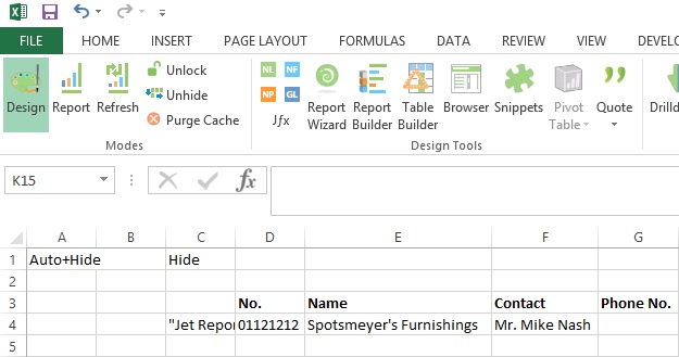
Let’s start with creating Option Page before we start with report creation:
NPGLUsage-1

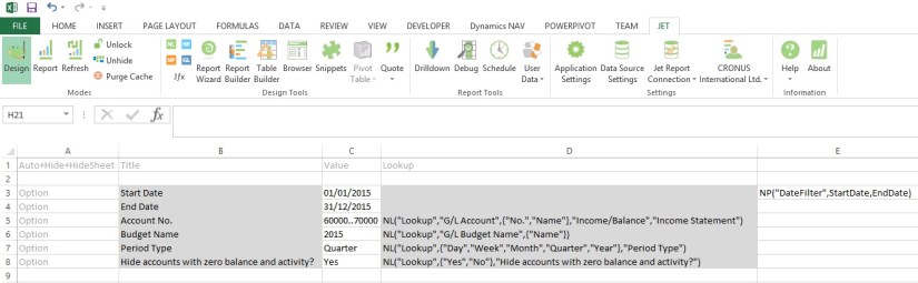
If you see in above sheet few filters are defined for the report, most of them are normal and Lookup which we have already discussed in previous report and posts.

Please be sure ‘=’ have been removed from formulas for presentation purpose, make sure you add them when use in your report.

Here new thing which we see is in E3 Cell:

=NP(“DateFilter”,StartDate,EndDate)

Here NP function creates a filter variable date filter which takes the StartDate & EndDate to create filter in Navision format like 01/01/2015..31/12/2015, which can be used in other Jet Functions as an parameter.

Option denotes these value will be asked from user when report is executed.

Lookup provides List of Values for selection to the user.

All text in A Column & Row 1 are the keywords or reserved words of the Jet Reports.

All text B3..B8 are Text or Option Heading which will be displayed in Option form when report is executed.

All text C3..C8 are the default Values for the options, remember (*) means no filters applied or include all. Don’t Forget to define Name of the cells in Name box, you will find this in the Left of the Formula Bar. The name I am using in my report defined below, this will help us using these user friendly name as filter in our Functions.

Cell Name
C3 StartDate
C4 EndDate
C5 GLAccountNo
C6 BudgetName
C7 PeriodType
C8 BlankZero
E3 DateFilter

Let’s Start our Report Design, Insert one more sheet for report format design.

Our design will be as follows, we will discuss the formula used in these columns later below in this post.

NPGLUsage-2

The Jet Formulas we are using in above sheet is as below:

Cell Formula
I3 =NL(,”Company Information”,”Name”)
J4 =PeriodType
J5 =NP(“DateFilter”,StartDate,EndDate)
J6 =NP(“Eval”,”=Today()”)
K8 =NL(“Columns=5”,NP(“Dates”,StartDate,EndDate,PeriodType))
K9 =NL(,NP(“Dates”,K8,”30/12/2050″,PeriodType,TRUE))
C12 =IF(AND(Heading=FALSE,BlankZero=”Yes”,MIN(K12:Q12)=0,MAX(K12:Q12)=0),”Hide”,”Show”)
D12 =NL(“Rows”,”G/L Account”,,”No.”,GLAccountNo,”Date Filter”,DateFilter)
E12 =NF($D12,”Account Type”)
F12 =OR(AccountType=”Heading”,AccountType=”Begin-Total”)
G12 =NF($D12,”Indentation”)
H12 =IF(E12=”Posting”,NF(D12,”No.”),IF(OR(E12=”Total”,E12=”End-Total”),NF(D12,”Totaling”),”0″))
I12 =REPT(” “,G12*5) & NF($D12,$I$11)
K12 =GL(“Budget”,$H12,ColumnStartDate,ColumnEndDate,,,,,,,BudgetName)
L12 =GL(“Balance”,$H12,ColumnStartDate,ColumnEndDate)

We can mix and match Excel formulas too to achieve data we require in our report especially any calculation of values from other cell values. You may find many of them is being used in this report too. You can apply formatting of Excel for better presentation of your reports. Sometime cell references to help in repeating the value to the cells and making available to access to upcoming cells when report is executed.

In Cell C1 [Hide+?] denotes this column will be used to get decision at run time like if we want to hide or show the respective row. As this value will not be available at design time, but when report is executed some rows we want to hide from the output of the report to user. Anything we are sure and know well in advance that this row need to be Hide we can key [Hide] in column A of that Row.

See in Cell C12 formula: [=IF(AND(Heading=FALSE,BlankZero=”Yes”,MIN(K12:Q12)=0,MAX(K12:Q12)=0),”Hide”,”Show”)]

Here decision is taken either we need to Show/Hide this row from output depending upon the test value. This value will be only available when data is retrieved and presented in Report, at design time we cannot predict what will be the value in these column and what will be the result of our test.

If we want to Hide any Row we Key [Hide] in A Column of that Row, Similarly if we want to Hide any Column we Key [Hide] in Row 1 of that Column.

Column L8 & L9 simply copy Value of K8 & K9 Respectively. K10 =K8 here too value is copied.

Rest All Values are Simple text used for Heading in Report Output.

[=REPT] this is Excel Formula Repeats text a given number of times. Use REPT to fill a cell with a number of instances of a text string.

Syntax: REPT(text, number_times)

The Cell M12 usage simple Excel Formula [=K12-L12].

The Cell N12 also usage simple Excel Formula [=IF(K12=0,””,ROUND((M12/K12),2))]

On executing the Report I fill below Filters:

NPGLUsage-3

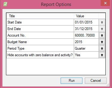
Applying above Filters the Output of report from my Standard Navision 2015 Report I get below Output:

NPGLUsage-4

Due to size limit I have reduced the zoom of the excel so that the exact report output in full can be shown.

Remain tuned for more information.

I will come up with more details in my upcoming posts.

Development Tips, Excel, How To, Jet Reports, Office Integration, Report

Using GL Function in Jet Reports

Syntax: =GL (What,Arg1,Arg2,Arg3,..,Arg22)

Purpose: Returns the budget, balance, net change, quantity, debits or credits of the G/L Account of a given company based on filters.

Dynamics NAV Parameter Description
 What NAV: Determines what the GL Function returns. Options are Balance, Budget, Quantity, Credits or Debits Note that the options available for the What argument depend on the Where argument.
 Account NAV: G/L Account Number, Filter or Range. If you specify a single, totaling account, you will get totals. If you specify multiple accounts or a range of accounts, totaling accounts will not be included in the returned number even if the other account(s) have nothing to do with the specified totaling account(s). If the Where argument is “Rows”, “Columns”, or “Sheets”, then the What options are “Accounts” which will give a list of account numbers, “Categories” which will give a list of account category numbers, or “SegX” where X is a segment number and which gives a list of that specific account segment.
StartDate NAV: Specifies the starting date of transactions to include. If you are interested in the balance of an account on a given date, leave StartDate blank. If you are interested in the net change of an account, use Balance and specify both the StartDate and EndDate
 EndDate NAV: Specifies the ending date of transactions to include. Specifying a start period and an end period will give you the net change between the first day of the start period and the last day of the end period. Specifying a start period with no end period will give you the net change between that start date and the present. Specifying no start period will give you the balance/budget as of the end period. Specifying no start period or end period will give you the present balance/budget.
 View NAV: The G/L Analysis View to use. Leave this blank to use balances from the G/L directly. Analysis Views are available in Navision version 3 and later. This field should be blank if you are using objects from an earlier version of Navision.
 Dim1 NAV: Filter for the first dimension of the analysis view. If View is blank, this is the filter for Global Dimension 1. Dimension totaling is handled the same way as Account totaling. In Navision versions before 3.0, Dim1 is used as the Department filter.
 Dim2 NAV: Filter for the second dimension of the analysis view. If View is blank, this is the filter for Global Dimension 2. In versions before 3, this is the Project filter.
 Dim3 NAV: Filter for the third dimension of the analysis view.
 Dim4 NAV: Filter for the fourth dimension of the analysis view.
 BusinessUnit NAV: Filter for the business unit.
 Budget NAV: Budget filter. This is unused unless returning budgets.
 Company NAV: Company Name. This must be spelled the same as it appears in Navision, including case, spaces and punctuation. If this parameter is empty (“”), the default company in the Jet Reports Options/Data Sources Screen is used.
 Reserved NAV: Blank. For backwards compatibility, a Data Source Name as defined in Jet/Options can be used.
 Reserved GP: Specifies filters for specific account segments. You can use either an account argument or segment filters, not both.
 Reserved GP: Specifies filters for specific account segments. You can use either an account argument or segment filters, not both.
 Reserved   GP: Specifies filters for specific account segments. You can use either an account argument or segment filters, not both.
 Reserved GP: Specifies the budget filter, blank for all budgets. Note that budgets are associated with a specific year in Great Plains so if your budget and fiscal year filters do not coincide you will get a 0 value.
 ExcludeClose NAV: “True” to exclude closing date transactions. Defaults to “False”.
 ShowQuery NAV: “True” to show the finhlink string that will be used for drilldown. Defaults to “False”.
 Reserved GP: Company name. If this parameter is blank, the default company is used.
 Data Source Data source name. If this parameter is blank, the default data source is used.

Reports based on the G/L are easy with the GL function.

=GL(What, Account, StartDate, EndDate, View, Dim1, Dim2, Dim3, Dim4, BusinessUnit, Company, Reserved, ExcludeClose, Reserved, Reserved, Reserved, Reserved, Reserved, Reserved, ShowQuery, Reserved, DataSource)

NAV Cronus Examples

To retrieve the balance of G/L account 44100, you would type the following.

=GL(“Balance”,”44100″)

If you wanted to know the net change of account 44100 between 1/1/2002 and 1/31/2002, you would type the following.

=GL(“Balance”,”44100″,”1/1/02″,”1/31/02″)

For G/L Balances with standard NAV:

  • you can filter on the two Global Dimensions for G/L Balances or
  • if using a NAV Analysis View, you can filter on up to 4 dimensions that are tied to that View=GL(“Balance”,”40100″,,,,”USA”,”COPPER”) 
  • Please note that some NAV verticals that allow more than 2 Global Dimensions may not be compatible with the GL function. 
  • For the balance of account “40100” with Global Dimension 1 of “USA” and Global Dim 2 of “COPPER”, you can use the following function.

Stay tuned for how to use GL Function in Jet Reports.

I will come up with more details on this in my upcoming posts.