Dear friends, I have published couple of posts on this topic. I will be adding more advanced features and details related to this in my upcoming posts.
For your ready reference below I present Links to those posts.
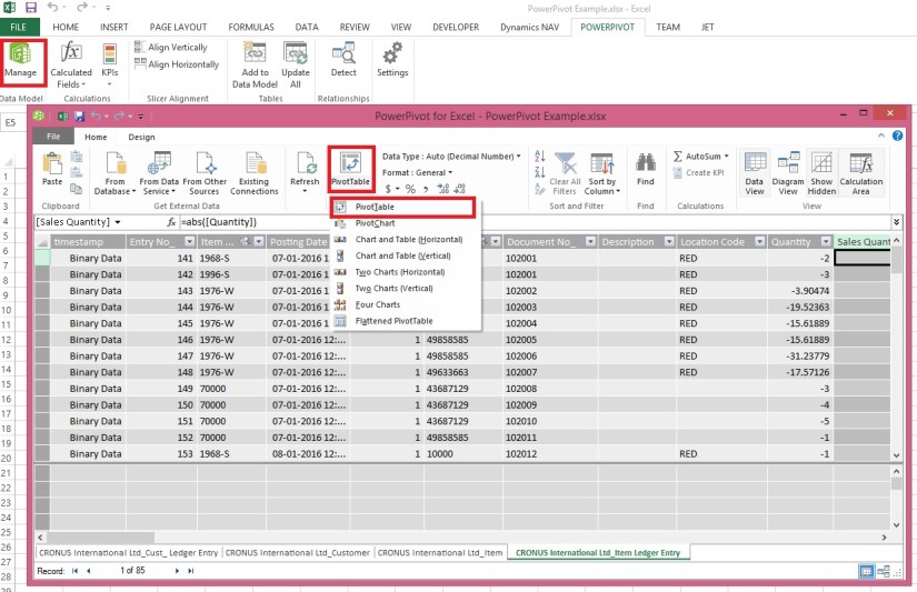
Start the Power Pivot in Microsoft Excel add-in
Troubleshooting: Power Pivot Ribbon Disappears
PowerPivot Creating a Data Model in Excel 2013
Adding more tables to the Data Model using Existing Connection – In PowerPivot
Add relationships to Data Model in PowerPivot
How to add Filter for data retrieval in PowerPivot Data model.
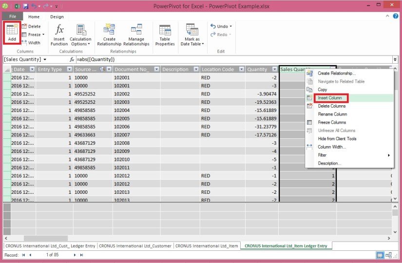
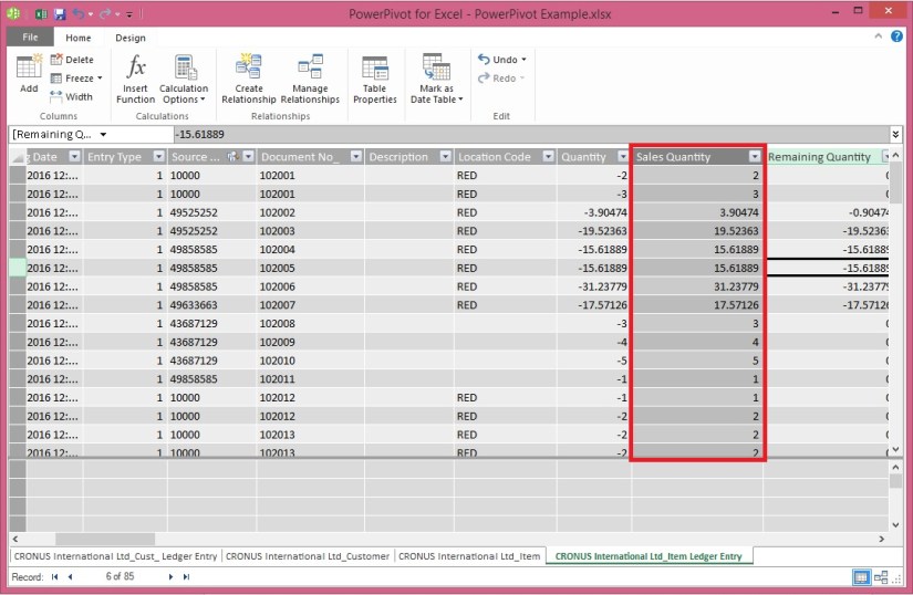
Create a calculated column in PowerPivot
Creating My First Report using PowerPivot
In Excel 2013, PowerPivot and Power View are no longer separate add-ins that need to be downloaded and installed. These add-ins are natively included.
PowerPivot in Excel 2013 is functionally very similar to the PowerPivot add-in for Excel 2010.
PowerPivot is an add-in that lets end users gather, store, model, and analyze large amounts of data in Excel. Power View provides intuitive data visualization of PowerPivot models and SQL Server Analysis Services (SSAS) tabular mode databases.
If you’re unfamiliar with either PowerPivot or Power View, I encourage you to first review my previous post links provided above to understand the basics.
Some parts of the PowerPivot architecture is embedded inside of Excel 2013.
- The PowerPivot version in Excel 2013 no longer uses a separate PowerPivot Fields list. Instead, the built-in PivotTable Fields list is used. This means that some capabilities from the Excel 2010 add-in (e.g., searching for fields by name, creation of slicers from the field list, surfacing of column descriptions when hovering over a field) are no longer available.
- Workbooks with PowerPivot models are no longer limited to 2GB in size in Excel 2013. However, the 2GB limit still applies to workbooks that will be published to SharePoint.
- In Excel 2013, a refresh of a PivotTable or PivotChart will, by default, initiate a refresh of the underlying data connections in the Data Model. This is very different from Excel 2010, where a PivotTable refresh only re-queries the model. The new refresh behaviour can be changed by clicking Connections on the Data tab, selecting Properties, and clearing the Refresh this connection on Refresh All check box.
- Stay tuned for more information on this topic. Till then keep practicing & exploring.
- In Excel 2013, a Power View “report” is a worksheet rather than an .rdlx file. There’s no concept of multiple report views. Instead, multiple Power View worksheets can be created within a single Excel workbook.
Stay tuned for more information on this topic. Till then keep practicing & exploring.