Development Tips, Excel, How To, PowerPivot

Start the Power Pivot in Microsoft Excel add-in

Power Pivot in Microsoft Excel 2013 is an add-in you can use to perform powerful data analysis in Excel. The add-in is built into Excel, but by default, it’s not enabled. Here’s how you enable Power Pivot before using it for the first time.

  • Go to File > Options > Add-Ins.

In the Manage box, click COM Add-ins> Go
PowerPivot-26

  • Check the Microsoft Office Power Pivot in Microsoft Excel 2013 box, and then click OK. If you have other versions of the Power Pivot add-in installed, those versions are also listed in the COM Add-ins list. Be sure to select the Power Pivot add-in for Excel.

PowerPivot-27
The ribbon now has a Power Pivot tab
PowerPivot-28

Development Tips, Excel, How To, Office Integration, PowerPivot, Report

Creating My First Report using PowerPivot

In my earlier posts we have created the Data model for Analysis.

If you missed them you can follow below links to refresh all information.

PowerPivot for Excel

PowerPivot Creating a Data Model in Excel 2013

Adding more tables to the Data Model using Existing Connection – In PowerPivot

Add relationships to Data Model in PowerPivot

How to add Filter for data retrieval in PowerPivot Data model.

Create a calculated column in PowerPivot

We have learned basic actions, let’s create our first Report.

I will be creating Pivot Matrix Customer Vs Item Sales.

Open the Excel in which we created our Data model and imported our table data.
PowerPivot-21
Select PivotTable From Ribbon under Home Tab.
PowerPivot-22

Select New Worksheet or Existing Worksheet as per the case.
PowerPivot-23
You will see a Pivot is inserted, in right side you will find all the tables available in the Data model of this Worksheet.
PowerPivot-24

Design the Pivot as above screenshot.
The output of this report will be as below if executed without Date Filter.
PowerPivot-25
I will come up with more details and features of PowerPivot in my upcoming posts. Till then keep practicing and stay tuned for more details on this topic.

Development Tips, Excel, How To, Office Integration, PowerPivot, Report

Create a calculated column in PowerPivot

If you have missed earlier post, please walkthrough them for better understanding from below links:

PowerPivot for Excel

PowerPivot Creating a Data Model in Excel 2013

Adding more tables to the Data Model using Existing Connection – In PowerPivot

Add relationships to Data Model in PowerPivot

How to add Filter for data retrieval in PowerPivot Data model.

In Power Pivot, you can use Data Analysis Expressions (DAX) to add calculations. In this task, I will add simple Excel Formula =ABS (Quantity) in Item Ledger Entry Sheet. You can add formulas either simple calculation from two fields or referencing from other tables and sheet. I will come with more details on this in separate post.

  • In the Power Pivot window, switch to Data View.
  • Select the Item Ledger Entry table/ sheet.
  • Click Design > Add.

PowerPivot-18

Alternatively you can Add by selecting Column, Right Click and choose Insert Column as you do in Excel.

New Column Will be Added.

  • In the formula bar above the table, type the following formula. AutoComplete helps you type the fully qualified names of columns and tables, and lists the functions that are available. You can also just click the column and Power Pivot adds the column name to the formula.

In my case it is =abs([Quantity])

  • When you have finished building the formula, press Enter to accept the formula.

Values are populated for all the rows in the calculated column. If you scroll down through the table, you will see that rows can have different values for this column, based on the data that is in each row.

Rename the column by right-clicking and selecting Rename Column.
PowerPivot-19

  • Type Sales Quantity, and then press Enter.

Below is the Screen after populating the value post formula application to Calculated Column.
PowerPivot-20

I will come up with more details in my upcoming post, Till then keep practicing and stay tuned for more details and updates on this topic.

Development Tips, Excel, How To, Office Integration, PowerPivot, Report

How to add Filter for data retrieval in PowerPivot Data model.

Recall from previous posts we have added Item Ledger Entry Table to our Data Model of PowerPivot.

Adding more tables to the Data Model using Existing Connection – In PowerPivot

Add relationships to Data Model in PowerPivot

My requirement is to retrieve only records related to Sales.

We will apply filter on Entry Type field to value [1]-[Sales] this way Item Leger Entry Sheet will have only Sales Data.

To do this we will add this filter to the query used for data retrieval.
PowerPivot-15

Select the Sheet for table – Item Ledger Entry from bottom.

Click on Design Tab on Top.

Now From Ribbon choose Table Properties.

PowerPivot-16

Select Query Editor from Switch to.

Add the Filter to your query.

Save your Query.

PowerPivot-17

From Home Tab, Select Refresh from Ribbon.

On Success completion Close the window.

Now your Item Ledger Entry is populated with Fresh data as per the modified Query.

I.e: All Entries which have Entry Type = 1 [Sales].

I will come up with more details in my upcoming post, till then keep practicing and stay tuned for future updates & posts on this topic.

Development Tips, Excel, How To, Office Integration, Report

Add relationships to Data Model in PowerPivot

You can systematically create table relationships for all new tables that you import. If you’re sharing the workbook with colleagues, having predefined relationships will be appreciated if they don’t know the data as well as you do.

When creating relationships manually, you will work with two tables at a time.

For each table, you’ll choose columns that tell Excel how to look up/ join related rows in another table.

Recall from my previous posts I will be continuing the example from using same Data Model

PowerPivot Creating a Data Model in Excel 2013

Adding more tables to the Data Model using Existing Connection – In PowerPivot

With your Data model sheet opened
PowerPivot-14
Click on Diagram View in Upper Right Side as highlighted in above screenshot.

Window will switch to Diagram View as shown in above screenshot, showing all the tables available in the Data model.

Click No_ in Customer Table and Drag to Item Ledger Entry Table and release the mouse button pointing to Source No_ field, you will see the Link is Established between these two tables showing the Link via Arrow line.

Repeat above step again between Item->No_ and Item Ledger Entry -> Item No_ fields.

Now we have Established connection between these three tables Customer, Item & Item Ledger Entry.

I will come up with more option on this topic in my next post, till then start practicing and stay tuned.

Development Tips, Excel, How To, Office Integration, PowerPivot, Report

Adding more tables to the Data Model using Existing Connection – In PowerPivot

For Introduction please see PowerPivot for Excel

Recall from my earlier post we have created a connection to SQL Navision Database in my previous post.

PowerPivot Creating a Data Model in Excel 2013

I will be modifying same connection to include more tables to the Data model.
PowerPivot-10

Click on PowerPivot-> Manage.

From the PowerPivot Sheet click on Existing Connections.

This will open Connection Window Listing all available connection to PowerPivot for this Sheet.

Double Click the Connection in my case Nav2015DB_SQL_Connection.
PowerPivot-6

Select first option as we used in previous post and then Next for next Step.
PowerPivot-11
Select Item & Item Ledger Entry Tables and then Finish to import Data to the Sheet.
PowerPivot-12
On Success Click Close to return to Data Model Sheets.
PowerPivot-13

You will find two new sheets have been added to PowerPivot Sheet.

I will come up with more option on this topic in my next post, till then start practicing and stay tuned for more details & Updates on this topic.

Development Tips, Excel, How To, Office Integration, PowerPivot, Report

PowerPivot Creating a Data Model in Excel 2013

Before you can create a PivotTable, you’ll need some data. Let’s get some data from the Navision database.

In Excel, open a blank workbook.

PowerPivot-1

PowerPivot-2

You have several options for getting data from no of sources.

Recall from my earlier post where we accessed data using web service in Excel.

Viewing Page Data in Excel Using PowerPivot (OData)

Let us see what other options are available to us.
PowerPivot-3

In today’s Example I will be connecting with SQL but will access Navision 2015 Database.

Follow the Steps below:
PowerPivot-4

Give meaningful name to your connection in my case I have used Nav2015DB_SQL_Connection.

Select the SQL Server to which you wish to connect in my case I have used INDEL-AXT5283N1, basically this is the SQL Server installed on my Laptop.
PowerPivot-5

Specify the Login method, I am using Windows Authentication, if required you can use SQL Server Authentication. In later case you will have to specify your User Name & Password.

Select the Database to Connect, I have selected Demo Database NAV (8-0) Std. Database for Navision 2015.

Click the Test Connection button, If everything is ok you will get Connection Succeed Message, as shown in above screen shot.

Press Next for next step.
PowerPivot-6

In this screen you have option to either import data from Tables and Views or you can Write Query to fetch data for import.

In my case for this example I am importing data from tables.

Select option – Select from a list of tables and views to choose the data to import and Press Next for next step.
PowerPivot-7

I have Selected two Tables Cust. Ledger Entry & Customer.

Select Related Tables button ensure to select if any other tables related to this Table.

In my case not applicable. Click Finish to add data to the Data Model/ Import the data of these two tables.
PowerPivot-8
Select Close to return to Data Sheet imported after this operation.
PowerPivot-9
Here you see your Data for these two tables have been imported in two sheets.

What happened?

You might not have realized it yet, but you’ve just created a data model. It’s created automatically when you import or work with multiple tables simultaneously in the same PivotTable report. The model is mostly transparent in Excel, but you can view and modify it directly using the Power Pivot add-in. In Excel, the presence of a data model is evident when you see a collection of tables in the PivotTable Fields list. There are several ways to create a model.

I will come up with more details in my next post.

Development Tips, Excel, Office Integration, PowerPivot, Report

PowerPivot for Excel

Power Pivot: Powerful data analysis and data modelling in Excel

Power Pivot is an Excel add-in you can use to perform powerful data analysis and create sophisticated data models. With Power Pivot, you can mash up large volumes of data from various sources, perform information analysis rapidly, and share insights easily.

In both Excel and in Power Pivot, you can create a Data Model, a collection of tables with relationships. The data model you see in a workbook in Excel is the same data model you see in the Power Pivot window. Any data you import into Excel is available in Power Pivot, and vice versa.

How the data is stored

The data that you work on in Excel and in the Power Pivot window is stored in an analytical database inside the Excel workbook, and a powerful local engine loads, queries, and updates the data in that database. Because the data is in Excel, it is immediately available to PivotTables, Pivot Charts, Power View, and other features in Excel that you use to aggregate and interact with data. All data presentation and interactivity are provided by Excel; and the data and Excel presentation objects are contained within the same workbook file.

Power Pivot supports files up to 2GB in size and enables you to work with up to 4GB of data in memory.

Download PowerPivot for Excel

To determine whether you are using 32-bit or 64-bit software, look at the C:\Program Files folder.

Download x86\PowerPivot_for_Excel_x86.msi if you have only “C:\Program Files”. Both the operating system and Office 2010 are 32-bit.

Download x86\PowerPivot_for_Excel_x86.msi if you have both “C:\Program Files” and “C:\Program Files (x86)”, and the Excel.exe application file is found in “C:\Program Files (x86)\Microsoft Office\Office14”. The operating system is 64-bit, but the version of Office is 32-bit.

Download x64\PowerPivot_for_Excel_amd64.msi if you have both “C:\Program Files” and “C:\Program Files (x86)”, and the Excel.exe application file is found in “C:\Program Files\Microsoft Office\Office14”. Both the operating system and Office 2010 are 64-bit.

Install PowerPivot for Excel

  • Double-click the .msi file to start the Setup wizard. Click Run.
  • Click Next to get started.
  • Accept the license agreement, and then click Next.
  • Enter your name, and then click Next.
  • Click Install.

Click Finish.

Verify Installation

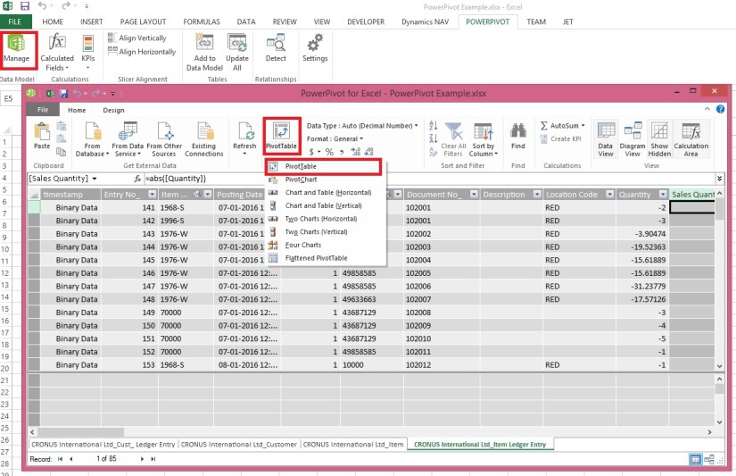
Start Excel. After you install the add-in, you can open the PowerPivot window by clicking the PowerPivot tab on the Excel ribbon, and then clicking PowerPivot Window.

An empty PowerPivot window opens over the Excel application window.

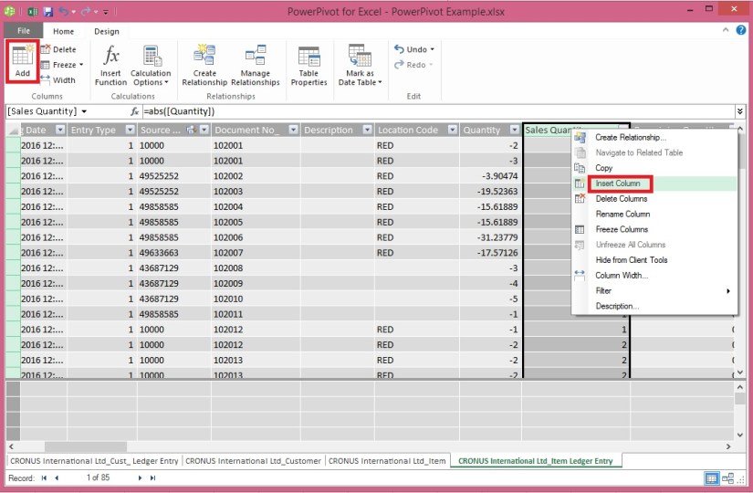
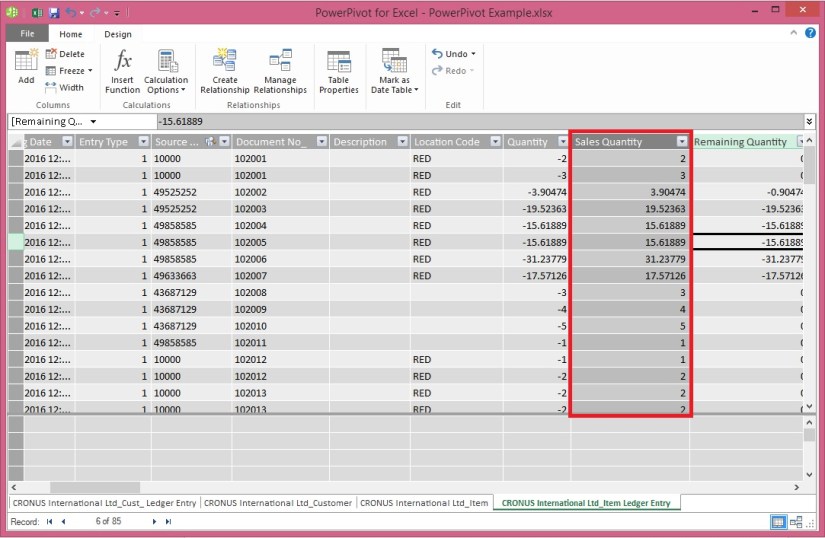
You can then use the Import Wizard to add tables of data, create relationships between the tables, enrich the data with calculations and expressions, and then use this data to create PivotTables and PivotCharts.

Stay tuned for more information in my upcoming posts.

Development Tips, Excel, Jet Reports, Office Integration, Report

Excel – Jet Report 2015 for Navision 2015

During the September month my most of the post was dedicated to Jet Reports.

There is many thing to share, which I will keep adding time to time.

For your reference here I present all the links related to this topic.

Jet Report for Excel – Navision 2015

Installing Jet Express for Excel – Navision 2015

Installing and Publishing the Jet Business Objects on the Microsoft Dynamics Server

Publishing the Jet Data Source Codeunit to the Web Service

Enable SOAP Services and identify connection parameters

Configuring a Data Source in Jet Express

Specify your Jet Interface Language

Uninstalling Jet Express

Using the Jet Ribbon Jet Essentials 2015 Update 1 for Navision 2015

Using Jet Report NL Function

Using Jet Report NF Function

Using Link in Jet Reports

Creating My First Report Using Jet Reports

Creating Simple List Report in Excel Using Jet Reports Part-1

Using NL( Lookup ) in Jet Reports Part-1

Creating Simple List Report in Excel Using Jet Reports Part-2

Using NL( Lookup ) in Jet Reports Part-2

Using NL( Lookup ) in Jet Reports Part-3

Using NP Function in Jet Reports

Using GL Function in Jet Reports

Creating Report in Jet Using NL, NF, NP & GL & Excel Formulas

Snippets in Jet Report

How to Use the Jet Report Scheduler

Other options for creating Report in Jet

Remain tuned I will be back with some other topics soon. I am just leaving this topic as of now but will keep adding more details on Jet reports time to time.

Development Tips, Excel, How To, Jet Reports, Office Integration, Report

Other options for creating Report in Jet

Jet Report

Report Wizard

An entire report can be created from a single table using the Report Wizard. The Report Wizard allows data to be grouped, filtered, sorted, subtotaled, and formated.


Report Builder

The Report Builder creates reports based on Jet Data Views.  Jet Data Views define table relationships, available fields, field captions, and table captions for a particular reporting area, such as sales, inventory, payroll, etc.  Jet Data Views can be created using the Data View Creator.

Before Using the Report Builder

Before you use the Report Builder you will need to import or create data views and categories.

A set of data views for Dynamics NAV can be found on Jet Web Site you can access the same from here. You can also click on the Download Data Views link within the Report Builder.

After downloading the file, you should open the .zip folder and extract the data view category (.jdc) file.

Importing Data Views and Categories

To import data views and categories, go to the Data Source Settings and select File -> Import -> Data View Categories.


Table Builder

An entire report can be created from a single or more table using the Report Wizard. The Table Wizard allows data to be grouped, filtered, sorted, subtotaled, and formated.


Browser

Provides browsing window to Select Tables and Fields, using which you can directly create an NL/ NF Function with their parameters and arguments.


This way I reach to end of my Jet Report Introduction Series. In future I will keep adding more details.