
Graduating from Reporting to Business Intelligence
Video-1
Video-2
Graduating from Reporting to Business Intelligence
Video-1
Video-2
The 5 Minute Dashboard – It’s Easier than You Think
Video-1
Video-2
Web Based Dashboards Provide Insight from Anywhere
Video-1
Video-2
During the September month my most of the post was dedicated to Jet Reports.
There is many thing to share, which I will keep adding time to time.
For your reference here I present all the links related to this topic.
Jet Report for Excel – Navision 2015
Installing Jet Express for Excel – Navision 2015
Installing and Publishing the Jet Business Objects on the Microsoft Dynamics Server
Publishing the Jet Data Source Codeunit to the Web Service
Enable SOAP Services and identify connection parameters
Configuring a Data Source in Jet Express
Specify your Jet Interface Language
Using the Jet Ribbon Jet Essentials 2015 Update 1 for Navision 2015
Creating My First Report Using Jet Reports
Creating Simple List Report in Excel Using Jet Reports Part-1
Using NL( Lookup ) in Jet Reports Part-1
Creating Simple List Report in Excel Using Jet Reports Part-2
Using NL( Lookup ) in Jet Reports Part-2
Using NL( Lookup ) in Jet Reports Part-3
Using NP Function in Jet Reports
Using GL Function in Jet Reports
Creating Report in Jet Using NL, NF, NP & GL & Excel Formulas
How to Use the Jet Report Scheduler
Other options for creating Report in Jet
Remain tuned I will be back with some other topics soon. I am just leaving this topic as of now but will keep adding more details on Jet reports time to time.

Report Wizard
An entire report can be created from a single table using the Report Wizard. The Report Wizard allows data to be grouped, filtered, sorted, subtotaled, and formated.
Report Builder
The Report Builder creates reports based on Jet Data Views. Jet Data Views define table relationships, available fields, field captions, and table captions for a particular reporting area, such as sales, inventory, payroll, etc. Jet Data Views can be created using the Data View Creator.
Before Using the Report Builder
Before you use the Report Builder you will need to import or create data views and categories.
A set of data views for Dynamics NAV can be found on Jet Web Site you can access the same from here. You can also click on the Download Data Views link within the Report Builder.
After downloading the file, you should open the .zip folder and extract the data view category (.jdc) file.
Importing Data Views and Categories
To import data views and categories, go to the Data Source Settings and select File -> Import -> Data View Categories.
Table Builder
An entire report can be created from a single or more table using the Report Wizard. The Table Wizard allows data to be grouped, filtered, sorted, subtotaled, and formated.
Browser
Provides browsing window to Select Tables and Fields, using which you can directly create an NL/ NF Function with their parameters and arguments.
This way I reach to end of my Jet Report Introduction Series. In future I will keep adding more details.
Overview
The Jet Scheduler is a powerful tool that allows users to schedule reports to be automatically run by the Windows Task Scheduler. The user can also control where the output file is saved to, if the report should be emailed once it has been generated, and the output format of the report.
Creating a New Scheduled Task
To set up a scheduled report, open the report in Excel, click the Jet ribbon, and click the Schedule button.

Click the New Task… button to schedule a new task.

The Scheduled Task window will now appear.
Reports Tab

The Reports tab contains general information about the scheduled task.
Schedule Tab

This tab will define the frequency of how often the report will be run as well as if the task is currently disabled and if the report should be run when the user is logged off.
The available options for the frequency are:
Frequency Tab

The name of this tab will change depending on the frequency specified on the Schedule tab.
In the screenshot above a Weekly frequency has been specified.
Email Tab

The Email tab allows the user to define who the report will be sent to if emailing is desired.
Output Tab
The Output tab allows the user to define how the file should be saved once it is finished running. This tab also enabled the user to turn on logging to troubleshoot errors with the Scheduler process as well as use Batch File Generation for the reports.

Remain tuned for more details, I will come up with more details and features in my upcoming posts.
Snippets are small, reusable report parts that can be shared between Jet users.
Configuring the Snippet Folder and Sharing Snippets
Snippets are stored in the “Jet Reports Snippets” folder located in your My Documents directory.
This location can be changed in the Application Settings. Each snippet is stored in a *.snippet file. To share snippets, copy the snippet files from one user’s snippet directory to another’s. Close and open the Snippets window and the newly added snippets will become available.

Creating and Using a Snippet
Creating a Snippet
To create a snippet, open the Snippet tool. Highlight the range of cells containing the piece of functionality for which to make a snippet. Then, click the New Snippet button in the Snippet tool.
I have created a simple Report for Active Customers, which Lists all the customers where Blocked = ‘’
We want to save this as a snipped so that any user can reuse it if required.

Using a Snippet
To use a snippet, drag and drop it from the Snippets window to any cell of your workbook. Any existing Excel formulas, text, or formatting in these cells will be overwritten.
Rename
You can rename a snippet by selecting it and pressing F2 or by right-clicking it and selecting Rename.
Delete
Delete a snippet by selecting it and then pressing the Delete button in the Snippet tool or by pressing the delete key.
Replace
You can replace the contents of the current snippet by selecting the region of the worksheet that you would like to use as the contents, selecting the snippet you wish to replace in the Snippet tool then pressing the Replace button.
Organizing Snippets
Snippets are organized in a folder structure. Snippets can be organized into folders using drag and drop or cut/copy/paste within the Snippet tool.
Will come up with more information and other features.
Dear friends today I will discuss report “General Ledger Budget to Actual by Period” and demonstrate the usage of NP & GL Functions.
This report will contain all the Functions, Commands we discussed till now and usage of NP & NL Functions.
You can refer my earlier posts for more detailed information which will help you understanding this report better, for your convenience I am providing link to previous posts which may help you understanding the terms being used in this report.
Using NL( Lookup ) in Jet Reports Part-1
Using NL( Lookup ) in Jet Reports Part-2
Using NL( Lookup ) in Jet Reports Part-3
Using NP Function in Jet Reports
Using GL Function in Jet Reports
Let’s start with creating Option Page before we start with report creation:
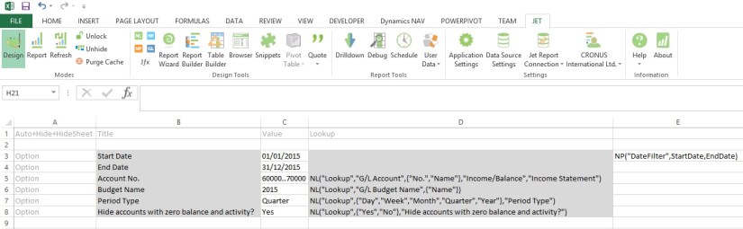
If you see in above sheet few filters are defined for the report, most of them are normal and Lookup which we have already discussed in previous report and posts.
Please be sure ‘=’ have been removed from formulas for presentation purpose, make sure you add them when use in your report.
Here new thing which we see is in E3 Cell:
=NP(“DateFilter”,StartDate,EndDate)
Here NP function creates a filter variable date filter which takes the StartDate & EndDate to create filter in Navision format like 01/01/2015..31/12/2015, which can be used in other Jet Functions as an parameter.
Option denotes these value will be asked from user when report is executed.
Lookup provides List of Values for selection to the user.
All text in A Column & Row 1 are the keywords or reserved words of the Jet Reports.
All text B3..B8 are Text or Option Heading which will be displayed in Option form when report is executed.
All text C3..C8 are the default Values for the options, remember (*) means no filters applied or include all. Don’t Forget to define Name of the cells in Name box, you will find this in the Left of the Formula Bar. The name I am using in my report defined below, this will help us using these user friendly name as filter in our Functions.
| Cell | Name |
| C3 | StartDate |
| C4 | EndDate |
| C5 | GLAccountNo |
| C6 | BudgetName |
| C7 | PeriodType |
| C8 | BlankZero |
| E3 | DateFilter |
Let’s Start our Report Design, Insert one more sheet for report format design.
Our design will be as follows, we will discuss the formula used in these columns later below in this post.

The Jet Formulas we are using in above sheet is as below:
| Cell | Formula |
| I3 | =NL(,”Company Information”,”Name”) |
| J4 | =PeriodType |
| J5 | =NP(“DateFilter”,StartDate,EndDate) |
| J6 | =NP(“Eval”,”=Today()”) |
| K8 | =NL(“Columns=5”,NP(“Dates”,StartDate,EndDate,PeriodType)) |
| K9 | =NL(,NP(“Dates”,K8,”30/12/2050″,PeriodType,TRUE)) |
| C12 | =IF(AND(Heading=FALSE,BlankZero=”Yes”,MIN(K12:Q12)=0,MAX(K12:Q12)=0),”Hide”,”Show”) |
| D12 | =NL(“Rows”,”G/L Account”,,”No.”,GLAccountNo,”Date Filter”,DateFilter) |
| E12 | =NF($D12,”Account Type”) |
| F12 | =OR(AccountType=”Heading”,AccountType=”Begin-Total”) |
| G12 | =NF($D12,”Indentation”) |
| H12 | =IF(E12=”Posting”,NF(D12,”No.”),IF(OR(E12=”Total”,E12=”End-Total”),NF(D12,”Totaling”),”0″)) |
| I12 | =REPT(” “,G12*5) & NF($D12,$I$11) |
| K12 | =GL(“Budget”,$H12,ColumnStartDate,ColumnEndDate,,,,,,,BudgetName) |
| L12 | =GL(“Balance”,$H12,ColumnStartDate,ColumnEndDate) |
We can mix and match Excel formulas too to achieve data we require in our report especially any calculation of values from other cell values. You may find many of them is being used in this report too. You can apply formatting of Excel for better presentation of your reports. Sometime cell references to help in repeating the value to the cells and making available to access to upcoming cells when report is executed.
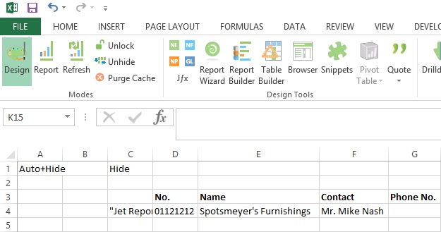
In Cell C1 [Hide+?] denotes this column will be used to get decision at run time like if we want to hide or show the respective row. As this value will not be available at design time, but when report is executed some rows we want to hide from the output of the report to user. Anything we are sure and know well in advance that this row need to be Hide we can key [Hide] in column A of that Row.
See in Cell C12 formula: [=IF(AND(Heading=FALSE,BlankZero=”Yes”,MIN(K12:Q12)=0,MAX(K12:Q12)=0),”Hide”,”Show”)]
Here decision is taken either we need to Show/Hide this row from output depending upon the test value. This value will be only available when data is retrieved and presented in Report, at design time we cannot predict what will be the value in these column and what will be the result of our test.
If we want to Hide any Row we Key [Hide] in A Column of that Row, Similarly if we want to Hide any Column we Key [Hide] in Row 1 of that Column.
Column L8 & L9 simply copy Value of K8 & K9 Respectively. K10 =K8 here too value is copied.
Rest All Values are Simple text used for Heading in Report Output.
[=REPT] this is Excel Formula Repeats text a given number of times. Use REPT to fill a cell with a number of instances of a text string.
Syntax: REPT(text, number_times)
The Cell M12 usage simple Excel Formula [=K12-L12].
The Cell N12 also usage simple Excel Formula [=IF(K12=0,””,ROUND((M12/K12),2))]
On executing the Report I fill below Filters:
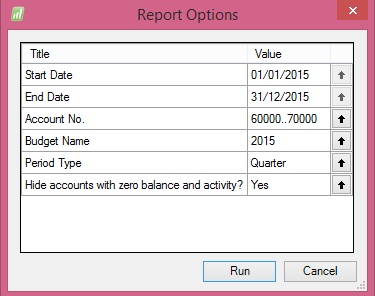
Applying above Filters the Output of report from my Standard Navision 2015 Report I get below Output:

Due to size limit I have reduced the zoom of the excel so that the exact report output in full can be shown.
Remain tuned for more information.
I will come up with more details in my upcoming posts.
Syntax: =GL (What,Arg1,Arg2,Arg3,..,Arg22)
Purpose: Returns the budget, balance, net change, quantity, debits or credits of the G/L Account of a given company based on filters.
| Dynamics NAV Parameter | Description |
| What | NAV: Determines what the GL Function returns. Options are Balance, Budget, Quantity, Credits or Debits Note that the options available for the What argument depend on the Where argument. |
| Account | NAV: G/L Account Number, Filter or Range. If you specify a single, totaling account, you will get totals. If you specify multiple accounts or a range of accounts, totaling accounts will not be included in the returned number even if the other account(s) have nothing to do with the specified totaling account(s). If the Where argument is “Rows”, “Columns”, or “Sheets”, then the What options are “Accounts” which will give a list of account numbers, “Categories” which will give a list of account category numbers, or “SegX” where X is a segment number and which gives a list of that specific account segment. |
| StartDate | NAV: Specifies the starting date of transactions to include. If you are interested in the balance of an account on a given date, leave StartDate blank. If you are interested in the net change of an account, use Balance and specify both the StartDate and EndDate |
| EndDate | NAV: Specifies the ending date of transactions to include. Specifying a start period and an end period will give you the net change between the first day of the start period and the last day of the end period. Specifying a start period with no end period will give you the net change between that start date and the present. Specifying no start period will give you the balance/budget as of the end period. Specifying no start period or end period will give you the present balance/budget. |
| View | NAV: The G/L Analysis View to use. Leave this blank to use balances from the G/L directly. Analysis Views are available in Navision version 3 and later. This field should be blank if you are using objects from an earlier version of Navision. |
| Dim1 | NAV: Filter for the first dimension of the analysis view. If View is blank, this is the filter for Global Dimension 1. Dimension totaling is handled the same way as Account totaling. In Navision versions before 3.0, Dim1 is used as the Department filter. |
| Dim2 | NAV: Filter for the second dimension of the analysis view. If View is blank, this is the filter for Global Dimension 2. In versions before 3, this is the Project filter. |
| Dim3 | NAV: Filter for the third dimension of the analysis view. |
| Dim4 | NAV: Filter for the fourth dimension of the analysis view. |
| BusinessUnit | NAV: Filter for the business unit. |
| Budget | NAV: Budget filter. This is unused unless returning budgets. |
| Company | NAV: Company Name. This must be spelled the same as it appears in Navision, including case, spaces and punctuation. If this parameter is empty (“”), the default company in the Jet Reports Options/Data Sources Screen is used. |
| Reserved | NAV: Blank. For backwards compatibility, a Data Source Name as defined in Jet/Options can be used. |
| Reserved | GP: Specifies filters for specific account segments. You can use either an account argument or segment filters, not both. |
| Reserved | GP: Specifies filters for specific account segments. You can use either an account argument or segment filters, not both. |
| Reserved | GP: Specifies filters for specific account segments. You can use either an account argument or segment filters, not both. |
| Reserved | GP: Specifies the budget filter, blank for all budgets. Note that budgets are associated with a specific year in Great Plains so if your budget and fiscal year filters do not coincide you will get a 0 value. |
| ExcludeClose | NAV: “True” to exclude closing date transactions. Defaults to “False”. |
| ShowQuery | NAV: “True” to show the finhlink string that will be used for drilldown. Defaults to “False”. |
| Reserved | GP: Company name. If this parameter is blank, the default company is used. |
| Data Source | Data source name. If this parameter is blank, the default data source is used. |
Reports based on the G/L are easy with the GL function.
=GL(What, Account, StartDate, EndDate, View, Dim1, Dim2, Dim3, Dim4, BusinessUnit, Company, Reserved, ExcludeClose, Reserved, Reserved, Reserved, Reserved, Reserved, Reserved, ShowQuery, Reserved, DataSource)
NAV Cronus Examples
To retrieve the balance of G/L account 44100, you would type the following.
=GL(“Balance”,”44100″)
If you wanted to know the net change of account 44100 between 1/1/2002 and 1/31/2002, you would type the following.
=GL(“Balance”,”44100″,”1/1/02″,”1/31/02″)
For G/L Balances with standard NAV:
Stay tuned for how to use GL Function in Jet Reports.
I will come up with more details on this in my upcoming posts.
Syntax: =NP (What, Arg1, Arg2,…,Arg22)
Purpose: Does various utility functions documented below.
Let’s see what options are available in below table:
| What | Description/Parameter |
| “Eval” | Evaluate the formula in the Arg1 parameter. The formula must be enclosed in quotes and will be evaluated when the report refreshes. |
| “DateFilter” | Calculates a date filter using the start date and end date specified in the Arg1 and Arg2 parameters. |
| “Union” | Returns (in the form of a Jet-specific list) the Union of two arrays specified in the Arg1 and Arg2 parameters. Note that in versions of Jet Essentials 2015 and earlier, if NP(“Union”) is by itself in a cell, it will only return the first value from the array. For those versions, you must put it inside an NL(“Rows”) in order to correctly return all the data. |
| “Integers” | Returns a string that can be used to generate integers using a Replicator, where Arg1 is the start number and Arg2 is the end number. |
| “Intersect” | Returns (in the form of a Jet-specific list) the intersection of two arrays specified in the Arg1 and Arg2 parameters. Note that in versions of Jet Essentials 2015 and earlier, if NP(“Intersect”) is by itself in a cell, it will only return the first value from the array. For those versions, you must put it inside an NL(“Rows”) in order to correctly return all the data. |
| “Difference” | Returns (in the form of a Jet-specific list) the difference of two arrays specified in the Arg1 and Arg2 parameters. Note that if NP(“Difference”) is by itself in a cell, it will only return the first value from the array. You must put it inside an NL(“Rows”) in order to correctly return all the data. |
| “Format” | Formats an expression with a specific Excel formatting string. Arg1 is the expression to format such as a date or cell reference, and Arg2 is the Excel formatting string such as “YYYY/MM/DD” for a date formatted with a 4-digit year then a 2-digit month and 2-digit day. |
| “Join” | Joins the elements of the array specified in Arg1 together into a single string separated by the contents of Arg2. |
| “Split” | In versions of Jet Essentials 2015 Update 1 and higher, this function splits the string in Arg1 into a Jet-specific list. |
| In earlier versions of Jet Essentials, this function splits the string in Arg1 into an array of values. The splitting is delimited by the contents of Arg2. Note that if NP(“Split”) is by itself in a cell, it will only return the first value from the array. You must put it inside an NL(“Rows”) in order to correctly return all the data. | |
| “Codeunit” | Evaluates and returns the value returned by the Dynamics NAV code unit function. |
| “Companies” | Returns a list of the companies associated with a data source. Arg1 is a company filter such as A* to return all companies that start with the letter A. Leaving Arg1 blank will return all companies. Arg2 is the data source. Leaving Arg2 blank will return companies from the current data source. Note that you should reference the result of this function in the table argument of an NL replicator function to actually list them out in Excel. |
| “Dates” | Returns a string that can be used to generate dates using a Replicator, where: |
| Arg1 is the start date | |
| Arg2 is the end date. | |
| Arg3 can be used to specify a period type of Day, Week, Month, Quarter, or Year. Default is Day. | |
| Arg4 can be set to “True” in order to return the end of each period. Default is “False”. | |
| “DataSources” | Returns an array containing the current user’s Jet data sources. |
| “Formula” | Evaluates the Excel formula contained within Arg1. |
| “Slicer” | Returns an Excel Slicer in Arg1 that can be used as a filter in Jet functions when using a Cube data source. |
EVAL
To increase performance, you can reduce cross-sheet references. The following NP evaluates the formula in cell of D5 from a worksheet called Options. =NP(“Eval”,”=Options!$D$5″)
This function is executed once on refreshing the report, rather than for every cell update. =NP(“Eval”,”=Today()”)
Performance can also be increased by not using volatile functions.
DATEFILTER
Results of using the NP(DateFilter) function, which can then be nested in other functions.

INTEGERS
This NP(Integers) function will create rows with the numbers 1 through 10. =NL(“Rows”,NP(“Integers”,1,10))
JOIN
The following NP(Join) joins the strings from an array and creates the result “100|200|300|400” for potential use in another function. =NP(“Join”,{“100″,”200″,”300″,”400″},”|”)
SPLIT
The following NP(Split) splits up the string “this|is|an|array” and creates the array {this, is, an, array}. =NP(“Split”, “this|is|an|array”, “|”)
COMPANIES
The following NP(Companies) function lists all the companies for the current data source in rows. =NL(“Rows”,NP(“Companies”))
DATES
The use of NP(Dates) to create a set of column headers for a report. (Dates can also be placed in reverse order by putting the later date in first)

DATASOURCES
This NP(DataSources) function will return a list of the data sources in use on the machine it is run on. =NL(“Rows”,NP(“Datasources”))
FORMULA
Used in conjunction with the NL(Table) function to define a calculated column in the table definition. For example: To determine available credit for a customer; if cell E6 contains the credit limit, and cell F6 contains the open credit, then =NP(“Formula”,”=E6-F6″) would be put in the field list of the NL(Table) definition
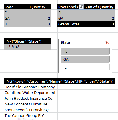
SLICER
The Slicer function works in conjunction with pivot tables and dashboards to provide information for filters when refreshing reports.
Array Calculations
Arrays are lists of data values. You can obtain a string representing such a list from Jet using “Filter” as the What parameter in an NL function. The values in arrays returned by Jet are guaranteed to be unique. The resulting array might be a list of Customers or a list of Invoice Document numbers or any other list of data that match a set of filters. The array calculation operations of the NP function allow you to find different combinations of two arrays.
An example of when you would need an array calculation is listing the invoice document numbers where either the Type on an Invoice Line is “Item” for all item numbers, or the Type is “G/L Account” and the account number is 300. Both the Item numbers and the G/L Account numbers are stored in the same “No.” field, so there is no single set of filters that will create this list of document numbers.
The array operations available in the NP function are “Difference”, “Union” and “Intersect”. The difference between two arrays consists of all of the elements that are in the first array but are not in the second. The union of two arrays consists of a single copy of all of the elements in both arrays with any duplicates eliminated. The intersection of two arrays is the set of elements that are common to both arrays. An example of the results of the array operations are listed in the table below.
| Array 1 {100, 200, 300, 400, 500} | Array 2 {400, 500, 900, 1000, 2000} |
| Difference | {100, 200, 300} |
| Union | {100, 200, 300, 400, 500, 900, 1000, 2000} |
| Intersect | {400, 500} |
=NL(“Rows”, NP(“Union”, NL(“Filter”,”Customer”,”No.”,”Name”,”A*”), NL(“Filter”,”Customer”,”No.”,”Name”,”B*”)))
=NL(“Rows”,”Customer”,”No.”,”Name”,”A*|B*”)
The following formula creates a list down rows of the document numbers of all invoices where either the Type field is “Item”, or it is “G/L Account” and the No. field is 2000.
=NL(“Rows”, NP(“Union”, NL(“Filter”,”Sales Invoice Line”,”Document No.”,”Type”,”Item”), NL(“Filter”,”Sales Invoice Line”,”Document No.”,”Type”,”G/L Account”,”No.”,”2000″)))
You should be cautious using arrays because they are often not the easiest or fastest way to solve a problem. Example 1 is a good example of a query that does not require arrays, and will run much slower if you use them. Also remember that, with Jet Essentials 2015 and earlier, if NP(“Union”), NP(“Intersect”), or NP(“Difference”) are by themselves in a cell they will only return the first value from the array. You must put them inside NL(“Rows”) as in the examples above in order to correctly return all the data.
There are two more array operations that behave a bit differently than those listed above: “Split” and “Join”. “Split” takes two text strings and splits the first string based on the second, resulting in an array. For instance, if you wanted to create a list of account numbers based on the string “1000+2000+3000”, the formula would look like the following.
=NP(“Split”,”1000+2000+3000″,”+”)
The result would be the array {“1000″,”2000″,”3000”}. Note that this must be put inside an NL(“Rows”) as in the Union examples above in order to return all the data.
In the opposite scenario, if you have an array but would like to create a text string by joining each element of that array separated by a given string, you would use the “Join” operation. Using the same array, you can create a string for a filter with array values separated by the “|” character with the following formula.
=NP(“Join”,{“1000″,”2000″,”3000″},”|”)
The result would be the text string “1000|2000|3000”, which is a valid filter that you could pass into an NL function.
For Join and Split, Arg1 of the NP function is the value you want to manipulate and Arg2 is the character by which you want to join or split the value. If you experiment with these operations, you will find that you have an amazing amount of flexibility, especially when you use them in conjunction with the other array calculation formulas listed above.
Please note that the results of an NP(“Join”) may be very large and thus putting it directly inside another function may cause problems with Excels 256 character formula limit as in the following formula.
=NL(“Rows”,NP(“Split”,NP(“Join”,{“some”,”array”,”here”},”|”),”|”))
It is recommended that in a situation like this the NP(“Join”) be placed in a separate cell as in the following.
B2: =NP(“Join”,{“some”,”array”,”here”},”|”)
B3: =NL(“Rows”,NP(“Split”,B2,”|”),”|”))
Stay tuned for usage of NP functions in Jet Reports.
I will come up with more details in my upcoming posts.

You must be logged in to post a comment.